An arsonist sets a fire at a car dealership that kills a sales person. The name of an extremist environmental group is spray-painted on the scene, but the group denies involvement. It becomes Don's task to determine whether the group or someone else is responsible.
Charlie and Larry are called in for help and use statistical data analysis techniques to try and figure out if there is a pattern to the fires that would help provide a profile of the arsonist
Statistics is a the branch of mathematics that studies collections of data, providing a way of analysing it, interpretating it and presentating it. While Charlie uses its techniques in a crime scene investigation, it is actually used in a wide variety of scientific or science-related fields.
One of the most basic uses of statistical methods is to provide people like Charlie with means of summarizing and describing large or complex sets of data; this is called descriptive statistics. In more advanced situations, patterns in the data may be even modeled so as to account for randomness in the observations, and then used to draw inferences about the process or population being studied; this is called inferential statistics.
We will focus in this lesson on the first kind of uses, and we will explore a few ways of summarizing large collections of data, starting with the most obvious ones.
| Length of scorch marks l | Rate of burn r |
| 1.0 | 4.3 |
| 1.2 | 4.5 |
| 2.2 | 4.9 |
| 1.4 | 5.6 |
| 1.4 | 3.9 |
| 1.1 | 4.1 |
| 1.8 | 3.9 |
| 1.9 | 4.9 |
| 2.1 | 5.0 |
We will investigate some basic operations that can still extract valuable information from a given collection.
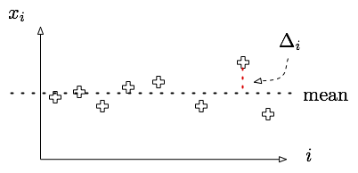
Given a collection of samples x1, ..., xn, one can forme the mean of the samples using by taking the average of all the xi's. That is to say, mean =  .
.
The mean of a collection of samples by itself doesn't always reflect the right notion of "average" sample value. The mean salary of a baseball player in the majors leagues, for example is $1.2 million dollars. Only given this fact, it is easy to see how the perception of the overpaid baseball player was created.
However, it is often conveniently ignored that the median salary for major leaguers is only $410,000, where the median is the "middle" salary for baseball players: 50% make more than $410,000, but 50% make less.
Suppose now you are given a collection of samples (xi, yi) describing the distribution of height and weight in a classroom. One might wonder whether there is any relationship between those two variables, meaning how accurate is it to guess someone's weight knowing their height, for example.
One measure of such a relationship between two variables can be found by computing the covariance and the correlation factor of the two variables. If xbar and ybar are the mean x and y values respectively, then the covariance and the correlation factor are given by:


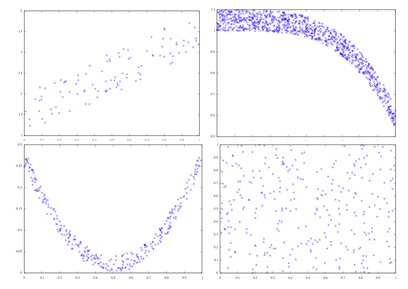
The higher the correlation function, the more linear relationship there is between the two variables. Covariance and correlation have to be taken with a grain of salt as their meaning is much more subtle than first appears.
This webpage does a really good job showing that correlation and coveriance do not tell the full story, and thus one should be careful drawing conclusions solely based on their values.
Wikipedia is always a good source of information, and in this case, provides very interesting plots that coulp help understand these two notions.
Linear regression is a very widely used technique whose purpose is to find linear trends in large chunks of data. It is used to find the line that best approximates a collection of numerical data points (x1, y1), ..., (xn, yn). Doing that, its reduces the complexity of the data into 2 numerical parameters that specify the approximating line: something like y = 2 x + 3. It can also be used to predict an y-value given an x-value that is not in the samples. This approximating line is also called least squares line.
Suppose we have a collection of a thousand pairs of fire properites, such as the average length of scorch marks and the amount of gasoline remnants, and we would like to reduce this collection of data to 2 parameters by finding the best approximating line in the following sense:
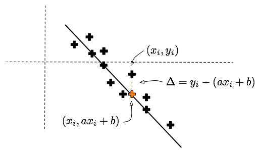
Given a line y = a x + b, and a sample (xi, yi), we can calculate the vertical error between that point and the line. This error is given by
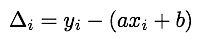
If we sum the squares of these errors over all the samples, we get a function of a and b that encodes how far a given line is from being a good approximation to the sample points. The smaller E(a,b), the better the approximation is.

In the next activity, we investigate how to find the values of a and b that realize the minimal error.
 and
and  , then find
  and
and  and are zero. Show that this is equivalent to
  and
and 

In the following application, we explore some examples and applications of this technique.
| Diameter D in km | Frequency F |
| 32-45 | 51 |
| 45-64 | 22 |
| 64-90 | 14 |
| 90-128 | 4 |
| 1/D2 | Frequency F |
| 0.001 | 51 |
| 0.0005 | 22 |
| 0.00024 | 14 |
| 0.000123 | 4 |
Is a line a reasonable approximation now? Find the least mean squares line and write F = a * (1/D)2 + b