
Knot theory
III. Fundamental concepts of knot theory (continued)
Recall our primary goal in knot theory:
How can we distinguish two knots?
We have seen several examples in the previous two lessons. Before looking at our goal directly, we need to have some necessary mathematical tools in our hands. This is exactly the content of the lesson here. It turns out that it is useful, first, to project the knot onto a two-dimensional plane. This is the content of section 1.
Section1. Regular diagram
As usual, we always think of a knot sitting in space. To be more precise, a knot is in a 3-dimensional space that we are living in. So, we are able to assign coordinates P(x,y,z) to every point on the knot, as an indication of the position of the point in our 3-dimensional space. Let us denote by p, the map that projects the point P(x,y,z) onto the point P'(x,y,0) in the xy-plane, see fig. 24.
fig. 24.
If K is a knot (or link), we shall say that p(K)=K' is the projection of K. Further, if K has an orientation assigned, then in a natural way K' inherits its orientation from the orientation of K. However, K' is not a simple closed curve lying on the plane, since K' possesses everal points of intersections. But by performing several elementary knot moves on K, intuitively this is akin to slightly shifting K in space, we can impose the following conditions on these projections :
(1) K' has at most a finite number of points of intersection.
(2) If Q is a point of intersection of K', then the inverse image of Q back in K has exactly two point. That is, Q is a double point of K', see fig. 25(a), it cannot be a multiple point of the kind shown in fig. 25(b).
(3) A vertex of K (the knot considered now as polygon) is never mapped onto a double point of K'. In the two examples in fig. 25(c), 25(d), a polygonal line projected from K comes into contact with a vertex point(s) of K', so both of these cases are not permissible.

fig. 25
A projection that satisfies the above conditions is said to be a regular projection.
Throughout these lessons, we will work exclusively with regular projections, and to simplify matters, we shall refer to them just as projections, we will draw a distinction only if some confusion might otherwise arise. However, even if we restrict ourselves to (regular) projections, there are still a considerable number of them. Secondly, and at this juncture of quite some importance, is the ambiguity of the double points. At a double points of projection, it is not clear whether the knot passes over or under itself. To remove this ambiguity, we slightly change the projection close to the double points, drawing the projection so that it appears to have been cut. Hopefully, this will give a trompe l'oeil effect of a continuous knot passing over and under itself. Such an altered projection is called a regular diagram. See fig. 26(a), fig26(b).
A regular diagram gives us a sense of how the knot may in fact lie in 3-dimensions, that is, it allows us to depict the knot as a spatial diagram on the plane. Further, we can use the regular diagram to recover information lost in the projection, for example, in fig. 26(c), it is the projection of the two non-equivalent knots in fig. 26(a) and fig. 26(b).
.PNG)
.PNG)
.PNG)
fig. 26
Therefore, we need to be a bit more precise with regard to the exact nature of a regular diagram and its crossing (double) points, since from the above description a regular diagram has no double points. The crossing points of a regular diagram are exactly the double points of its projection, p(K), with an over- and under- crossing segment assigned to them. Henceforth, we shall think of knots in terms of this diagrammatic interpretation, since, as we shall see shortly, this approach gives us one of the easiest ways of obtaining insight and hence results into the nature of knots.
For a particular knot (or link), K, the number of regular diagrams is innumerable. To be more exact, there is only one regular diagram of a knot, K, in our 3-dimensional space. However, from our discussion in the previous lessons, the knot K and a knot K' obtained from K by applying the elementary knot moves are thought of as being the same knot. So, we can think of the regular diagram of K' as being a regular diagram for K. Hence, it follows that for K, the number of regular diagrams is innumerable.
It is possible that a regular diagram may have crossing points of the type shown in fig. 27(a), fig.27(b).

fig. 27
More generally, suppose two regular diagrams of two knots (or links) are connected by a single twisted band. We can, in fact, remove this 'central' crossing point by applying a twist, either to the left or right, to the knot. A regular diagram that does not possess any crossing points of this type is called a reduced regular diagram.
Exercise 3.1 Show that a regular diagram for K1*K2 can be obtained by placing the regular diagrams of the oriented knots K1 and K2 side by side, and connecting them by means of two parallel segments, see fig. 28 for an example.

fig. 28
Section2. What is a knot invariant?
As a way of determining whether two knots are equivalent, the concept of the knot invariant plays a very important role. The types of knot invariants are not just limited to, say, numerical quantities. These knot invariants can also depend on commonly used mathematical tools, like polynomials.
Suppose that to each knot, K, we can assign a specific quantity q(K). if for two equivalent knots the assigned quantities are always equal, then we call such a quantity, q(K), a knot invariant. This concept of assigning some mathematical quantity to an object under investigation is not limited just to knot theory, it can be found in many branches of mathematics.
We knot that if a knot K and another knot K' are equivalent, then it is possible to change K into K' by applying elementary knot moves to K a finite number of times. Therefore, for a quantity q(K) to be a knot invariant, q(K) should not change as we apply the finite number of elementary knot moves to the knot K. It follows from this, for example, that the number of edges of a knot is not a knot invariant. The reason is that elementary knot moves (recall: the definition of elementary knot moves is in lesson 2, section1) either increase or decrease the number of edges. Similarly, if we consider the size of a knot, it is not an invariant as well since the size of a knot changes when we apply the elementary knot moves.
A knot invariant, in general, is unidirectional, that is:
if two knots are equivalent, then their invariants are equal.
For many cases the reverse of ' if...then... ' does not hold. In contraposition, if two knot invariants are different then the knots themselves cannot be equivalent, and so a knot invariant gives us an extremely effective way to show whether two knots are non-equivalent. The history of knot theory may be said to be an account of how the various knot invariants were discovered and their subsequent application to various problems. To find such knot invariants is by definition a 'global' problem. On the other hand, to actually calculate many of these knot invariants, which we shall discuss a bit later, is quite difficult. Further, to find a method to calculate these invariants is also a 'global' problem.
Notice that it is still an open problem in knot theory to find a complete knot invariant. There is no known complete knot invariants at this stage. By 'completeness', what we mean here is that the reverse of the above statement 'if two knots are equivalent, then their invariants are equal. ' holds. More concretely speaking, for any two given knots, if the knot invariants of these two knots are equal, then these two knots are equal. If this condition is satisfied, we call such a knot invariant complete. Put it in the other way, a complete knot invariant means a complete classification of the set of all knots in our space, up to equivalence.
Section3. Reidemeister moves
A knot (or link) invariant, by its very definition, as discussed in the previous section, does not change its value if we apply one of the elementary knot moves. It is often useful to project the knot onto the plane, and then study the knot via its regular diagram. If we wish to pursue this line of thought, we must now ask ourselves what happens to, what is the effect on, the regular diagram if we perform a single elementary knot move on it? This question was studied by K. Reidemeister in the 1920s. In the course of time, many knot invariants were defined on Reidemeister's seminal work. In this section, we are going to study the moves defined by him, called the Reidemeister moves.
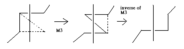
A solitary elementary knot move, as might be expected, gives rise to various changes in the regular diagram. However, it is possible to restrict ourselves to just the four moves (strictly speaking, changes) shown in fig. 29 and their inverse moves, also in fig. 29:

fig. 29
That these moves may, in fact, be made is reasonably straightforward to understand. For example, M2 may be thought of as the move that corresponds to an elementary knot move on a regular diagram, which replaces, AB by (AC)U(CB), as shown in figure 30.

fig. 30
Exercise 3.2 Verify that, in fact, M3, M4 are possible, that is, they are a consequence of some finite sequence of elementary knot moves.
Definition 3.1 If we can change a regular diagram, D, to another D' by performing, a finite number of times, the operations M2, M3, M4, and/or their inverses, then D and D' are said to be equivalent. We shall denote the equivalence between D and D' by D=D'.
These three moves M2, M3, M4 and/or their inverses are called the Reidemeister moves. Notice that after making any elementary knot moves to the original knot, the regular diagram remains essentially unchanged by making suitable (sequences of) Reidemeister moves corresponding to the elementary knot moves we have made. That is, we may state the following theorem:
Theorem 3.1 Suppose D and D' are regular diagrams of two knots (or links) K and K', respectively. Then,
K=K' if and only if D=D'
We may conclude, from the above theorem, that the problem of equivalence of knots, in essence is just a problem of the equivalence of regular diagrams. Therefore, a knot (or link) invariant may be thought of as a quantity that remains unchanged when we apply any one of the above Reidemeister moves to a regular diagram. In the following, we shall often need to perform locally a finite number of times a composition of Reidemeister moves, for simplicity we shall call such a composition an R-moves.

fig. 31
Theorem 3.2 The moves shown in fig. 31 are R-moves.
Proof: For the upper picture :
For the lower picture :
.bmp)
Exercise 3.3 Using similar methods as in theorem 4.2, show that the following moves are R-moves.

In the next lesson, we shall explain several knot invariants that have played substantial role in research into knots.