Knot theory
VII. Applications
In this lesson, we aim at explaining some applications of knot theory. Although knot s are ubiquitous in nature, we may still wonder why knot theory is important in mathematics. So we are going to discuss a few things in mathematics that are related to knot theory. Afterwards, we try to briefly explain the connections between knot theory and biology, a seemingly surprising relation discovered by the scientists in the recent years.
Section 1. Knot and graph
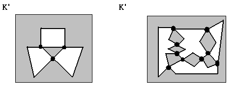
Suppose D is a regular diagram for a knot K and K' is a projection of K. We can think of K' as a graph on the plane. The vertices of the graph correspond to the crossing points of K. See fig. 53.
fig. 53 Two K' as the a graph in the plane.
We can examine our graphs on the plane more closely. K' divides the plane into several domains. Starting with the outmost domain, we can colour the domains either grey or white. By definition, we shall colour the outermost (unbounded) domain grey. In fact, we can colour the domains so that the neighbouring domains are never the same colour, that is, on either side of an edge the colours never agree. (Why is it possible? Can you guess why?) Next, choose a point in each white domain, we shall call these points the centres of the white domains. If two white domains have crossing points in common, then we connect the two centres of of the white domains by edges. Each edge corresponds to a common crossing point respectively. In this way, we obtain the plane graph G from K' , see fig 54 for two plane graphs G corresponding to the two K' in fig. 53.

fig. 54 These are the two plane graphs G obtained by the above descriptions from the two K' s in fig. 53.
Exercise 7.1 By the above method, check that the two G s obtained from fig. 53 are the correct ones.
However, in order for the plane graph to embody some of the characteristics of the knot, we need to use the regular diagram rather than the projection. So, we need to consider the under-crossings and over-crossings at a crossing. We can try to assign a sign + or - on each edge, for either an under-crossing or an over-crossing. More concretely speaking, we can do it in the following way, see fig. 55
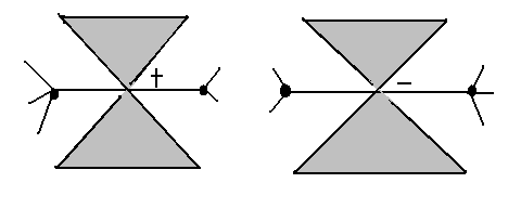
fig. 55 Notice that the horizontal edge in each picture is the edge passing through the crossing (corresponding to the edge in fig.54)
After assigning + or - in the graph, we have the refined (signed) plane graph for the two plane graphs in fig. 54, see fig. 56.
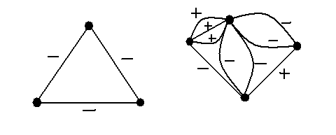
fig. 56 two refined plane graphs corresponding to those two in fig. 54
Conversely, we can construct from an arbitrary signed plane graph G a knot diagram:
To construct the subsequent knot, first place a small 'x' at the centre of each edge of G, see fig. 57 (b). From the endpoints of one of these of 'x', draw four lines that follow along the edges of G until they reach the endpoints of a neighbouring 'x'. What should start to appear if this prcocess is carried out at each 'x' is a projection of a knot, but with no information with regard to the nature of the crossing points, fig. 57 (c). Now, we can colour the planar domains (obtained from the partition of the domain by the newly-formed projective diagram) either black or white using the same method to decide which colour to apply as discussed previously. We may ascertain, and hence draw in the relevant crossing point information from the signs of the original graph. Obviously, the black and white colouring information disappears once the crossing point information is added and hence we obtain the required knot diagram, see 57 (d).
Therefore, for each signed plane graph there exists a corresponding regular diagram of knot ( see the correspondence between fig. 57(a) and fig. 57(d) ) . However, it is NOT necessarily true that the two different plane graphs give rise, by means of the above process, to two non-equivalent knots. It is still an open problem in knot theory.
.bmp)
.bmp)
.bmp)
.bmp)
fig. 57
The above approach was originally one of the methods used to construct a table of regular diagrams of all knots starting with the graphs with a relatively small number of edges and then increasing the number of edges. In this manner, Tait and Little produced an almost complete table of regular diagrams of knots with up to 11 crossing points. In recent years, this table has been amended and increased to include knots with up to 13 crossings.
In fig. 58, we provided the connected plane graphs with up to 4 edges and their corresponding knots (and links). The number of edges is equal to the number of crossing points of the regular diagram of the knot. Since, for the sake of clarity, we have not assigned signs to the edges so they are not regular diagrams of knots but rather their projections.
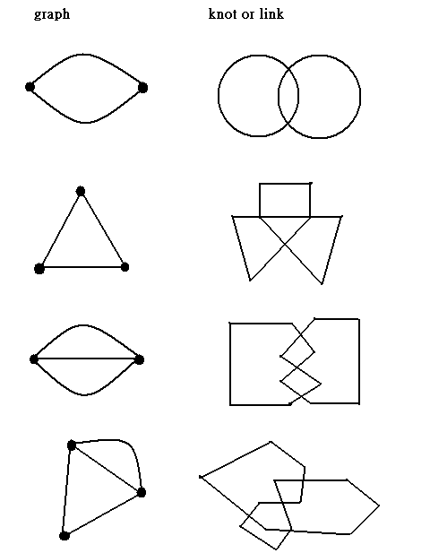
fig. 58
Exercise 7.2 Check that the above correspondence between plane graphs and knots (or links) are the correct ones.
Section 2. Knot and biology
F. H. C. Crick and J. D. Watson, in one of the most remarkable insights of the 20th century, unraveled the basic structure of DNA. For this profundity into the substance of living matter, they were jointly awarded the Nobel Prize for Medicine in 1962. Essentially, a molecule of DNA may be thought of as two linear strands intertwined in the form of a double helix with a linear axis. A molecule of DNA may also take the form of a ring, so it can become knotted or tangled. Further, a piece of DNA can break temporarily. While in this broken state the structure of the DNA may undergo a physical change, and finally the DNA will recombine. In fact, in the early 1970s it was discovered that a single enzyme called a topoisomerase can facilitate this complete process, from the initial break to the recombination. To put all the above in mathematics, knot theory is an essential tool.
A mathematical model for a DNA molecule is usually a thin, long, narrow(oriented) twisted ribbon, in fig. 59.
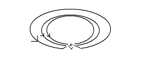
fig. 59
The two curves that form the boundaries of the ribbon represent the closed DNA strands. Notice that we also fix the orientation of the two curves, so we can consider it as an oriented link. And hence, by lesson 5, we have the link invariant the linking number for these two curves. Its change has an very important effect on the structure of the DNA molecule. For example, if we reduce the linking number of a double-strand DNA molecule, then the effect is to cause the DNA molecule to twist and coil, i.e. it is called supercoiling. More generally, recent research has shown that the knot type, or DNA molecule has an important effect on the actual function of the DNA molecule in the cell. Therefore, by using knot theory technique, it may be possible to gain further insight into the structure of a DNA molecule.
To end this discussion, we can take a look at the process of recombination at certain places in the knot, in fig. 60.
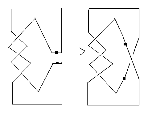
fig. 60 The process of recombination takes place in the DNA molecule, notice that there is a change in knot type in the knot.