Formally,
the dividend yield is equal to the ratio between
the annual dividend per share and the price per share. For example, if
the price per share is $100, the stock is paying quarterly $1 of
dividends per share and the dividend payments are not
reinvested in the stock, the annual dividend per share and
dividend yield would be equal to $4 and 4%, respectively.
Sometimes
secure, stable and low-growth companies distribute a portion of their
earnings to some of their share holders because they do not have to
reinvest them to sustain growth. These are known as
dividends
and are usually quoted in terms of the dollar amount each share
receives. When trading foreign currency, there exists an interest rate
paid per unit of the currency lent or borrowed, analogous to the
riskless
interest rate,
r, considered in the
binomial
model. This interest rate can be considered as a
dividend
yield (see tangent). In this lesson we will explore how the
previously developed theory changes when the risky asset in the market
has dividend payments. For simplicity, the examples presented below are
one-step models, however, the results easily extend to the multi-period
case.
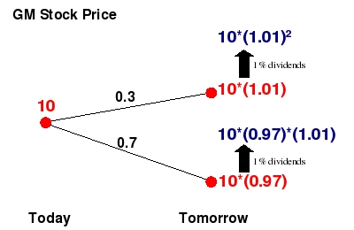
Example:
General Motors with dividend
Suppose the
stock price of GM is as in
example
3 of the second lesson. But now assume that we know that the
company will pay dividend at some point between today and tomorrow
(this is a very unrealistic assumption considering the current crisis
that "The Big Three" automakers, General Motors, Chrysler and Ford are
facing). We consider our time horizon to be 1 day and assume that the
dividend payment is 1% of the amount in dollars invested in the stock.
Also, as in example 3, we suppose that the riskless interest rate is
2%. The dividend payment between today and tomorrow has an effect on
the price of the stock by pushing it up by 1% as shown in the figure
below.


We have then
that
d'< r=0.02 < u', and according
to
activity
2 of lesson 3,
in this
case the market is arbitrage free.Activity
1
Explain why in this case the strategy:
short
one unit of the risky asset and invest $10 in the money market account
in no longer an arbitrage opportunity. What is the
risk
neutral probability q*
in this case.
Example:
Dollar Vs. Euro
In
example
2 we assumed that investors can borrow or lend Euro with no
interest rate. Clearly, this assumption is not realistic and it is
important to revise this example when the interest rate in Europe is
not supposed to be 0. Suppose now that the interest rate in Europe is
the same as it is in the US, namely 10%. If this is the case, the
arbitrage opportunity described in example 2 is no longer an arbitrage
opportunity: if you
short
one Euro and lend $1.5, tomorrow you will get $1.65 but you will owe
1.1 Euro. If the price of the Euro goes up, once you pay back your
debt, you will end up with a net loss of $(1.65*1.1)-$1.65=$0.165.
Hence the strategy of "going short on the Euro and long on the Dollar"
is not riskless and hence not an arbitrage opportunity anymore. The
natural question that arises then is: Is it possible to adjust this
strategy to get an arbitrage strategy? or, Is under these circumstances
the market arbitrage free?
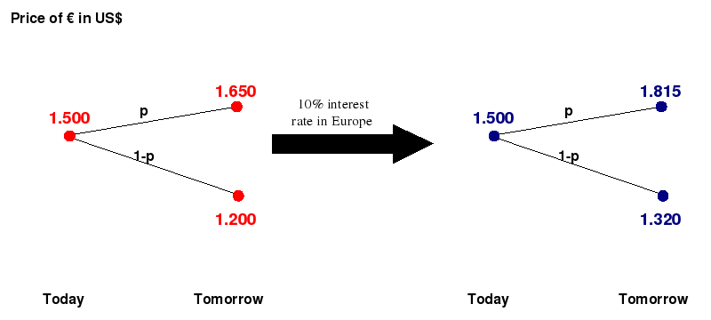
To answer this
question we reason as in the example above. The fact that the interest
rate in Europe is 10% is equivalent to saying that the price of one
Euro tomorrow is 1.1 times the price today. To account for this fact we
can redefine the price and rates of return of the "risky" Euro after
one period of time (see
the
binomial model and figure above):

We have then
that
d'< r=0.1 < u', and according to
activity
2 of lesson 3,
in this
case the market is arbitrage free.
Activity
2
In
activity
1 b) of the first lesson, we observed that when the interest
rate in the US is 5% and the interest rate in Europe is 0% then the
binomial model is arbitrage free. Explain why if the interest in Europe
were 31.25% the model would not be arbitrage free and exhibit an
arbitrage opportunity in this case.
The general case
In the examples above we assumed that the risky asset pays dividend as
a percentage of the value of the asset. Suppose that this percentage is
s. As we noticed above we can reduce the
problem to the one consider in
lesson
1 by adjusting the price of the risky asset and the rates of
return, namely

This very simple observation and
the
first fundamental theorem of asset pricing allow us to
conclude that in this case the market is arbitrage-free if and only if
d'<
r< u'.
Activity 3
-
Assuming that the interest rate r is fixed, under
what conditions on the dividend rate s the model is
arbitrage free?
- If the model is arbitrage free,
what is the risk
neutral probability q*
in terms of r and s?
- What is the fair price
you would have to pay today,
for 1 unit of the risky asset with delivery tomorrow? Discuss the
difference between the price when the stock pays no dividend and the
price you found. Hint: Use the probability q*
of part b) to calculate the price.
In the
multi-step case assuming that dividends are paid in every time
step and are all equal to
s% the
the
first fundamental theorem of asset pricing as proven in
lesson 3, states that
d'< r< u' is
also a sufficient and necessary condition for the multi-step model to
be arbitrage free. However, if dividends are not paid on a regular
basis, or are not equal, we can not utilize the binomial model as
presented in module 1 for our arguments. To cover this case, we refer
the reader to
lesson
9 where we study the case when the rates of return of the
risky asset are time dependent.