The Mole
Season 3, episode 4
In this episode, Charlie and the FBI team try to find a mole in the federal government that is leaking secrets to the Chinese.
Face Recognition
In this episode, Charlie uses a face recognition program to identify
the people that appear in a surveillance video. He uses a technique
called Eigenfaces to do this. Before understanding how this
technique works, we have to introduce a statistical technique
called Principal Component Analysis.
Principal Component Analysis
Principal Component Analysis or PCA is used to reduce
the dimensionality of a set of data. We will motivate PCA with a
simple example. Suppose that as a curious young scientist, you are interested in the properties of apples. You go to
the supermarket, buy 8 different apples, and then return home and
measure the volume and mass of each apple. Your results might look like this:
| Apple # | Mass | Volume
|
| 1 | 0.15 | 10.5
|
| 2 | 0.05 | 2.5
|
| 3 | 0.18 | 8.5
|
| 4 | 0.1 | 5.5
|
| 5 | 0.25 | 13.5
|
| 6 | 0.35 | 19.5
|
| 7 | 0.4 | 15.5
|
| 8 | 0.22 | 11.5
|
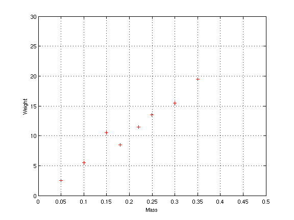
It is hard to notice any pattern in the data just by looking at the
table. However when the data is plotted on graph paper, it becomes
clear that the two measurements are related. In fact, they almost lie
along a straight line:
 Finding the pattern by drawing a graph worked because there were only
2 measurements per apple, and so the result was a 2 dimensional
graph. But what if instead we measured 10 features per apple? Then we
would need to draw a 10-dimensional graph to look for patterns.
That is clearly impossible -- when was the last time you found 10
dimensional graph paper??!!
Finding the pattern by drawing a graph worked because there were only
2 measurements per apple, and so the result was a 2 dimensional
graph. But what if instead we measured 10 features per apple? Then we
would need to draw a 10-dimensional graph to look for patterns.
That is clearly impossible -- when was the last time you found 10
dimensional graph paper??!!
Principal component analysis is a mathematical technique for finding
these patterns automatically. To apply the technique, we
use the following steps:
- Create a matrix X that contains all of the
measurements. Each row of the matrix corresponds to a single observation
and each column corresponds to a measurement.
- Compute the mean training vector by averaging together all of the rows of X. Call the mean vector u.
- Subtract u from every row of matrix X, to produce a new matrix Y.
- Compute the covariance matrix C of Y, using the following formula:

- Now we solve the following equation:
 where x is a vector and
  is a number. In general there
are many values of x and that make this equation
true. The possible values of are called
the eigenvalues of C, and the corresponding solutions
for x are called its eigenvectors.
is a number. In general there
are many values of x and that make this equation
true. The possible values of are called
the eigenvalues of C, and the corresponding solutions
for x are called its eigenvectors.
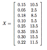
We will illustrate PCA by applying it to our apple example. In step 1 we create a matrix X storing all of the data. The matrix looks like this:
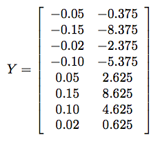
Then we compute the mean, which is u = (0.212,10.875). The result of step 3 is a new matrix Y where the mean has been subtracted off of every row of X:
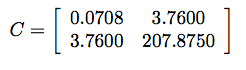
Step 4 gives us the following covariance matrix:
Finally, we compute the eigenvalues and eigenvectors.
The eigenvalues are about 208 and 0.003, and the
eigenvectors are (0.0181, 0.999) and (-0.999,0. 0181). The two
eigenvectors give us a new set of coordinates that explain the data
more compactly. That is, the results of PCA say that the data lies
mostly along the vector (0.0181, 0.999), since the corresponding
eigenvalue is so much larger than the other. In fact, if we extend
the vector (0.0181, 0.999) and overlay it on the graph of training
exemplars, we see that the majority of apples lie along the line:
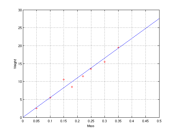 In other words, PCA gives us a new coordinate system that allows us to
represent the data more compactly instead of using the normal x- and
y- coordinate system. Since most of the apples lie along the line, we
can represent each apple with a single number -- its distance from the
origin along the line -- instead of the two numbers required by the x-
and y- coordinate system. PCA has given us a way to convert 2-dimensional data
to 1 dimension.
In other words, PCA gives us a new coordinate system that allows us to
represent the data more compactly instead of using the normal x- and
y- coordinate system. Since most of the apples lie along the line, we
can represent each apple with a single number -- its distance from the
origin along the line -- instead of the two numbers required by the x-
and y- coordinate system. PCA has given us a way to convert 2-dimensional data
to 1 dimension.
Eigenfaces
Now let us switch from apples to faces. Eigenfaces is a technique that
tries to reduce the dimensionality of face data, just like how we
reduced the dimensionality of apple data above.

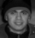
 To understand how eigenfaces work, we have to understand how images
are stored in a computer. A digital image is represented as a set
of pixels or points of light. For example, each of the face
images shown to the right is stored as a 40x40 grid of pixels, and
each pixel has a brightness value from 0 to 255. Mathematically, we
can think of an image as a vector of length 1600 (since 40*40=1600),
where each entry in the vector is in the range [0,255]. A specific
image is represented as a single point in this high dimensional space.
To understand how eigenfaces work, we have to understand how images
are stored in a computer. A digital image is represented as a set
of pixels or points of light. For example, each of the face
images shown to the right is stored as a 40x40 grid of pixels, and
each pixel has a brightness value from 0 to 255. Mathematically, we
can think of an image as a vector of length 1600 (since 40*40=1600),
where each entry in the vector is in the range [0,255]. A specific
image is represented as a single point in this high dimensional space.
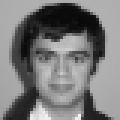
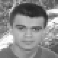
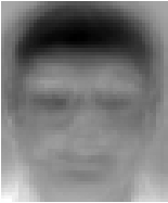
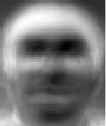
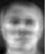
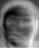
How would we go about comparing two face images to decide if they are
of the same person? One idea would be to compare the brightness
values of the two images pixel-by-pixel and to declare a match if all
of the pixel values were similar. We could accomplish this by
computing the Euclidean distance between the two points in the
high dimensional space. Unfortunately, this approach does not work,
because two pictures of the same person can be just different enough
such that no two pixels actually have the same value. For example, the
four images to the right are of the same person, but the pixel values
in every one of them are different.
In fact, virtually any two images of the same person are going to be
at least slightly different and thus be represented as different
vectors. It turns out that the number of possible images of the same
person is unbelievably large. Suppose we either add or subtract one
brightness value from every pixel in one of the above images. This
would change the image very slightly but the face would still be
recognizable. How many possible ways are there to do this? The answer
is 21600, or about 10480. This is an enormously large number; it is
many times more than the number of atoms in the universe!
Our approach suffers from what is called the curse of
dimensionality: we are representing our images in a way that is too
complicated. Our data has too many degrees of freedom compared to what
we need to accurately represent a face.
The technique Charlie uses to address this problem is called
Eigenfaces. The idea is to transform a face image into a much lower
dimensional space that represents only the most important parts of a
face. To apply the Eigenface technique, we first collect a training
set of many (hundreds or thousands) of facial images. Each of the
training images is represented as a vector of length 1600, as we saw
before. Then we create a matrix X that contains all of the
training vectors, one per row. The resulting matrix has size N x 1600,
where N is the number of training images. Then we perform PCA on the
matrix using the steps given above.
Just like before, PCA is used to reduce the dimensionality of the face
data. The result is a set of eigenvalues and eigenvectors, as before,
but researchers have given eigenvectors of faces a special name:
eigenfaces. Usually only a small number (e.g. 10) of eigenfaces are
kept after PCA is performed. Each of these eigenfaces is a sort of
"prototype" of some general face characteristics. Here are what some Eigenfaces look like:
Any given face can be encoded as a combination of these
eigenfaces. For example, your face might be 10% of the first
eigenface, 30% of the second eigenface, 60% of the third eigenface,
and 0% of the fourth. Eigenfaces thus lets us represent a face as a
point in low dimensional space, instead of the 1600-dimensional space
required before.
Face recognition
Now back to face recognition. Charlie has a
known database of face images, and a new query face that he wants to
find in the database. So he converts each of the images in the
database from 1600-dimensional space to 10-dimensional space using the
eigenfaces technique. He does the same with the new image. Then he can
compute the Euclidean distance between the new image and each known
image in the 10-dimensional "face space". The face image in the
database that has the lowest distance -- that is, the face that is
closest to the query image in "face space" is the person that he is looking for.
Activity 1
- Suppose you have a very simple camera that takes 10 x 10 pixel
images, and every pixel can take on one of only 2 brightness
values. How many possible images can your camera produce? If you were
to take two pictures randomly, what is the probability that the two
pictures would be exactly the same?
- Suppose you know that the eigenvalues of the following matrix are -1 and -2:
[ 0 1 ; -2 -3]
What are the corresponding eigenvectors?
Brachistochrone Problem. An upside down cycloid is the solution to the famous
Brachistochrone problem (curve of fastest descent) between two points; that is, the curve between two points that is covered in the least time by a body that starts at the first point with zero speed under the action of gravity and ignoring friction. This problem was solved posed in the
Acta Eruditorum, the first scientific journal of Germany, in 1696. The problem was solved by 4 famous mathematicians: Isaac Newton, Jakob Bernoulli, Gottfried Leibniz, and Guillaume de l'Hôpital.
Curtate cycloid
To determine that the woman was actually killed by a car instead of it being a hit-and-run, Charlie tries to describe walking in mathematical terms. He says "when you walk, it’s really a series of little circles rotating inside a larger circle. The heel orbiting backwards, then forward past the knee is a small
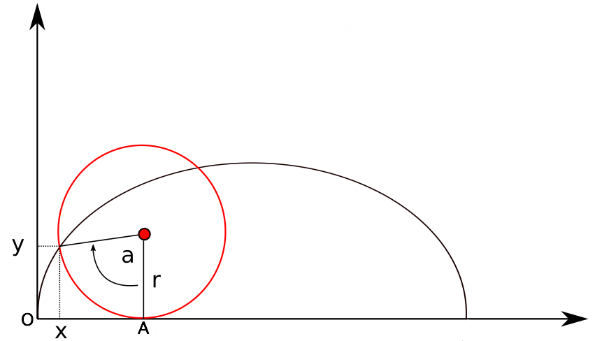
circle within the larger circle of walking." This movement can be thought of as a curtate cycloid, whose picture we include below.
In few words, it is the curve described by looking at the movement of a point on a circle while we move the circle along a straight line. In the activity below we study the mathematical equations that describe this curve
Activity 2: Equations of the cycloid.
- Consider the figure to the right and
argue that the distance between O and A is ra.
- Using the result from above, what is the value of x in terms of a and r? [Hint: Use trigonometric functions]
- What is the value of y? [Hint: Use trigonometry again]
- Compute the length of the segment of the curtate cycloid that has been drawn in the picture to the right.
Branching and Bounding
Charlie uses this combinatorial optimization technique to predict the next meeting between Carter and the Chinese.
Combinatorial Optimization Problems
Before describing this technique, we say something about combinatorial optimization problems. One such problem is the following "Find the pair of positive integers whose sum is 100, and whose product is as big as possible". In this case we are trying to maximize the two-variable function product of two integers, which is defined by f(x,y) = xy. f is called the objective function. Notice that the set S of non-negative integers in which we are interested is described by the equation x + y = 100. The set S is called the set of feasible solutions. In other words, a combinatorial optimization problem consists of these ingredients,
- The problem is to minimize a function f(x) of variables x1, x2 ..., xn over a region of feasible solutions S. That is, we are interested in finding
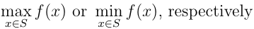
- The set S is usually determined by general conditions on the variables, such as them taking values on the non-negative integers.
In out example, we can just go ahead and try every single element in S to find which pair maximizes the objective function f. Of course there are many techniques to find the optimal solution, depending on the particular problem. Branching and bounding algorithms constitute one such technique.
B&B Algorithms
There exists a combinatorial optimization technique called branching and bounding (hereinafter called B&B) which basically consists of searching for the best solution among all possible solutions to a problem by dividing the set of solutions and using bounds for the function to be optimized. Since there is some enumeration of solutions involved in the process, this technique can perform very badly in the worst case; however, the integration of B&B algorithms with other optimization techniques and has proved useful for a wide variety of problems.
Here is a description of the three main components involved in
B&B algorithms for minimization problems (with the case for maximization problems dealt with similarly):
- A bounding function (upper or lower, depending on the case) g(x) for our objective function f that will allow us to discard some subsets of S.
- A branching rule that tells us how to divide a subset of S in case we are not able to discard such a subset as not having the optimal solution which we are looking.
- A strategy for selecting the subset to be investigated in the current iteration.
We describe the technique with the following example,
Example: Maximize the function Z = 21x1 + 11x2 given the constraints 7x1 + 4x2 ≤ 13 , with x1 and x2 non-negative integers.
Solution: The set S is described by the inequalities 7x1 + 4x2 ≤ 13, x1 ≥ 0, x2 ≥ 0. Since we cannot discard S, we subdivide it into smaller pieces, thus making the original problem smaller. For instance, let us focus on the subset of S where x2 = 0. Then Z attains its maximum when x1 = 13/7 (approx. 1.857). This first step was used as our branching rule, and now we focus on two subsets of S, S1 and S2 as shown in the picture below. We easily see that there are no feasible solutions on S2, and that the solution on S1 is Z = 37.5, which is attained with x1 = 1, and x2 = 1.5; this value of x2 is used as our new branching rule. We now consider the problem in two new subsets, S11 = {solutions with 0 ≤ x1 ≤ 1 and 0≤ x2 ≤ 1} and S12 = {solutions with 0 ≤ x1 ≤ 1 and x2 ≥2}. Solving the original problem (maximizing Z) for S12 yields Z = 37, which is attained by x1 = 0.71 and x2 = 2, so we branch at x2 once again and consider the sets {x1 = 1, x2 ≥ 2} and {x1 = 0 and x2 ≥ 2}. Finally, the solution must be in S11, and solving the original problem on this set yields Z = 32, which is attained by x1 = x2 = 1. Continuing in this matter, we obtain the answer Z = 33, which is attained when x1 = 0 and x2 = 3. This answer is in the set S1211

The picture above depicts the process used to solve our problem. We considered 9 subsets of S; that is, the number of vertices in the graph depicted above is 9.
Activity 3
- Using the procedure just explained, to maximize 2x + 3y, given that 10x + 3y ≤ 24, for non-negative integers x and y.
- Maximize -x + y, given that 12x + 11y ≤ 63, -22x + 4y ≤ -33, for non-negative integers x and y.
- * Let n be a positive odd integer. Consider the following optimization problem: Maximize -x0 subject to x0+2(x1+ ... + xn) = n, 0 ≤ xj ≤1 for j = 0, 1, ..., n, where all the variables are integers. Show that the number of subsets that need to be consider (number of vertices in the graph) is at least 2^[(n-1)/2].