Numb3rs 206: Soft Target
At numerous public facities throughout Los Angeles, the Department of Homeland Security is running training exercises to practice reacting to various terrorist activities. The first such training exercise takes place in the public underground transit system - and mid-training exercise, a real gas attack is unleashed in one of the railway cars. Although in the panic, little was seen of the movements of possible perpetrators, Charlie does manage to extrapolate where the gas bomb must have been released based on smoke diffusion patterns and predictive differential equations.
The basic math behind differential equations, diffusion equations, and fluid dynamics can be less than basic at best, but here are some activities and explorations to get a hands on feel of how these calculations can be done.
Ordinary Differential Equations:
Gas Diffusion? Differential Equations?
How is gas diffusion related to differential equations? Well, for starters, any time we know how fast "something" changes - grows, moves, disperses - and need to figure out a function desribing the configuration/position of our "something" at a particular time, we have a differential equation!
Scientists have long tied together the heat equation and the diffusion equation, as they are virtually identical models - one has particles of energy dispersing, the other, particles of matter!
A first-order, linear partial differential equation is an equation of the following form:
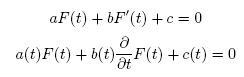
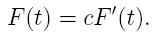
These are the same equation, although the latter emphasizes that my coefficients might also be functions of t, and that F'(t) is the first derivative of F(t) with respect to t.
These types of equations come up ALL the time in real-life applications. For example, in a basic case, if I know that the speed of my car is a constant 30 mph, and I start at mile 0 and go for t hours, where am I? Clearly, this should be F(t)=30t.
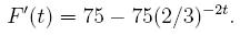
Similarly, if I am traveling 75mph at t=0, but my speed is decreasing by a third every half an hour, I need to solve the equation
Activity 1:
- Given G'(t)=20+36t+16t^4, solve for G(t) with the following initial conditions:
- G(0)=0
- G(1)=30
- G(2)=150
Remember that for differential equations of the form G'(t)=c(t), for some function c of t, we have from the Fundamental Theorem of Calculus that G(t) is the integral of G'(t) plus some constant!
- Solve the equation F'(t) above for F(t), assuming we started at the 10 mile marker.
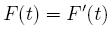
These are the most rudimentary of differential equations. A much more interesting example involves a relationship between the rate of chance F'(t) and our desired function F(t). For instance, if we want a neat equation, consider
While most of you know that the function we're looking for here is F(t)=e^t, how do we show this? Well, note that following steps 1-4, we see
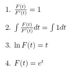
This proves a fact many of you knew - that our exponential function is its own derivative!
Activity 2:
Repeat the process above, but finding a solution for the equation
Let's look at one more cool and relatively basic ordinary differential equation before we move onward to the heat equation and other partial differential equations.
Consider a spring with a weight on the end of it. Our spring will vibrate up and down around an equilibrium point, and we can show (experimentally) that the spring will feel force proportial to how far away the weight is from this equilibrium point. Using Newton's Second Law of Motion, we know that the force a spring feels is proportional to its acceleration, so we have the following:
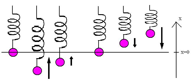
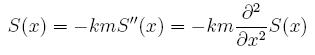
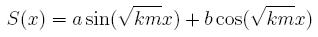
We need to find functions whose second derivatives are equal to some (negative) multiple of themselves. After some examination, we note that two functions that satisfy this are a*sin(rx) and b*cos(sx). Fiddling around with our equation above, we see that we should have
All we need do now is set our constants based on the initial conditions. As this is a "Second Order" Differential equation, we are going to need two different initial conditions - some velocity and some position.
Activity 3:
Solve for constants a and b (in terms of k, m, and x) for our spring model with the following initial conditions:
- At time t=0, the weight is traveling 5 m/s upward and passing through the equilibrium point.
- At time t=pi/2*sqrt(km), the weight is at 0 m/s, and at a position of 0.2 meters above the equilibrium point.
- At time t=pi/sqrt(km), the weight is going 1 m/s downward and at a position 0.1 meters above the equilibrium point.
The Heat/Diffusion Partial Differential Equations:
What's the difference between an "ordinary" and a "partial" differential equation (ODE and PDE respectively)? Well, the number of changing parameters (i.e. variables) mostly! To talk about heat or gas diffusion, we need a distribution function of time and position - as we need to know how hot (or dense) a given spot x is and how that changes over time. We will write this heat equation as F(x,t).
It can be shown that both diffusion and heat phenomena in one-spacial dimension (say, on a thin rod) can be described by the following partial differential equation in Cartesian, e.g. rectangular, coordinates:
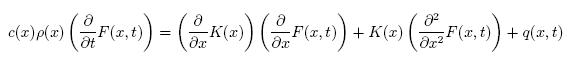
In this case, F(x,t) is our heat distribution as a function of time and position, p(x) is our mass density at x, c(x) is the specific heat of the material in the rod, and q(x,t) is an input source function (for example, a source of heat that might change in intensity or location over time.)
Looks complicated, right? Let's assume that we don't have a heat source and that our density and specific heat are constants across our entire 1-dimensional space. Our equation then reduces to something MUCH nicer:
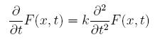
The constant k is called the "thermal diffusivity of the medium," and is equal to K/cp in our previous notation.
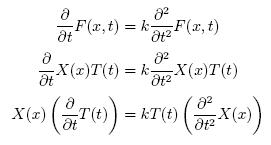
While I'm sure many of you let out a sigh of relief, we're not really out of the woods yet. What does this equation really say? Well, the change in our temperature distribution on our rod over time is proportional to how quickly temperature change is increasing or decreasing as we move through our material in the spacial dimension. Not very illuminating, eh? To really get a grip on a PDE, a standard technique is "separation of variables," which will help us reduce our problem in multiple variables to multiple problems in one variable at a time.
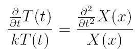
We assume that F(x,t) can be "separated," i.e. it can be written as F(x,t)=X(x)T(t). This may seem like a lot to assume. In practice however, if we can split our function this way, then solve for a solution, there are uniqueness theorems that guarantee that this isn't just right - it's the ONLY possible solution.
Let's plug this "separated" equation back into our original PDE:
So far, so good. Now we move everything that involves x to one side, and everything that involves t to the other side.
Activity 4:
The new equations on both sides of the equality symbol must be constant. Get into groups and brainstorm WHY.
We choose our new separation constant to be L, i.e.
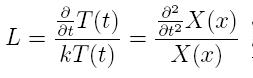
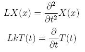
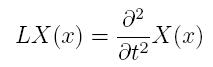
This will give us now the new ODEs that we will need to solve:
Activity 5:
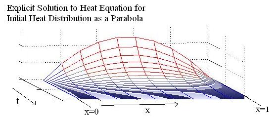
Given a uniform rod of length 1 with one end at x=0 and the other end at x=1, fix the ends of the rod at temperature zero. Give our rod an initial temperature distribution of f(x)=F(x,0). If the thermal diffisivity of the rod is k=1/5, work out the separation of equations in this case.
Given a second order ODE in X with conditions X(0)=0 and X(1)=0 that satisfies our first equation, namely,
we have a host of possible solutions. Since L isn't a fixed number, but instead, an eigenvalue, we note that for any
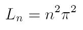
we have that
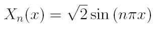
is a solution. These are the only possible eigenvalues and eigenfunctions, and they are "orthonormal" (if you know what that means!) Now that we know our possible Ln's, we need to try to figure out a Tn(t) for each of our Xn(x).
Activity 6:
Now we'll solve for our Tn given separation constants Ln. We saw that Ln had to be n^2pi^2, so we have that
Solve this to find the Tn which satisfy our equation for each eigenvalue Ln.
Fact:
We can now write our F(x,t) as a linear combination of these independent eigenfunctions, i.e.
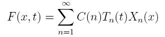
We've solved for Xn(x) and Tn(t), so now we have
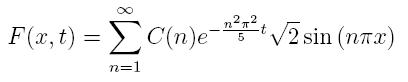
Given our initial heat distribution function f(x)=F(x,0), we set our C(n), and then we are done! Any f(x) can be our initial distribution, and the resulting F(x,t) will be the correct model!
References and Further Reading:
[1] P. DuChateau, D. Zachmann,
Applied Partial Differential Equations Dover Publications, 2002.
[2] L. Evans,
Partial Differential Equations (Graduate Studies in Mathematics, V. 19) GSM/19, American Mathematical Society, 1998.
[3] G. Articolo,
Partial Differential Equations & Boundary Value Problems with Maple V Academic Press, 1998.
[4]
Heat Equation
[5]
Partial Differential Equations