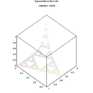
Exponential plotter on the 0-cell(download and open in Maple or view code here. The input "m" stands for a0. This plots the exponential function on the 0-1 blowup of the Sierpinski gasket on the 0-cell. The previous limit converges rapidly, so the 4 blowups approximation used here is the same graph for values of a0 less than -1. Also,a program for plotting along the diagonal is here.)
Julia set 0-0 Blowup plotter(download and open in Maple or view code here. This program needs some explaining. It blows up the 0-cell with a0=3+sqrt(3) any even number of times you wish. This eigenvalue is doubly periodic. The input "z1" is the q0 function value, z2 the q1 value, z3 the q2 value, and d half the number of zoom outs the program will do.)
Julia set 0-1 Blowup plotter(download and open in Maple or view code here. Same parameters and idea as the same one, except now it does the 0-1 blowup. Rotate the graphs to see cool pictures.)
Error on the 0-cell(download and open in Maple or view code here. This program plots Ea(x+q1)+Ea(x)/a0 on the 0-cell. In the proof that the general definition of the exponential converges, the fact that this function is on the order of 1/a02 is used. The behavior of this was used for a check for the calculations. The parameter "m" is the a0 value.)
Logarithm of the E function(download and open in Maple or view here. This graphs the logarithm of the E function, and appears to be linear. The parameter "m" stands for a0.)
Finally, here's a more efficent version of the first program. This one runs in Matlab. Thanks to Andrew Jonathon Marks of Cornell University for making this.
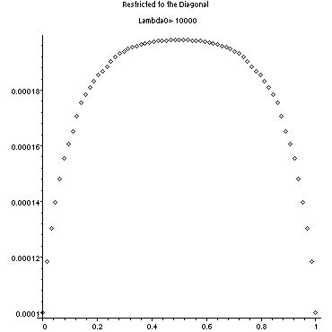
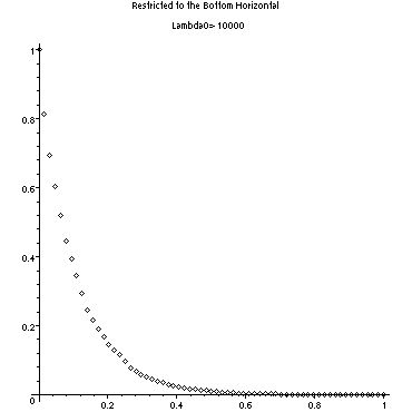
Here are pictures which will give an idea of what the E function looks like:
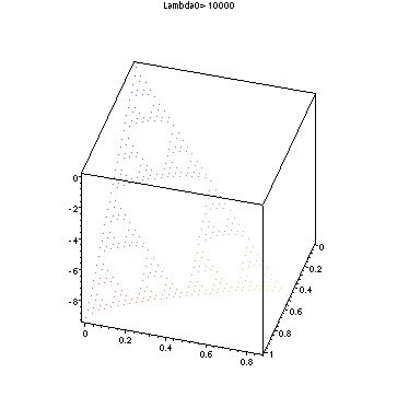
As a0 becomes larger, the flatter the top of the second graph becomes, and the closer the function is to behaving like the expnential on the real line. This can be checked by plotting the logarithm of the function like so:
I also used the third and fourth programs to make a plot of the blowups with doubly periodic graph eigenvalues. For the 0-1 blowup where a0=3+sqrt(3), a2n=3+sqrt(3) and a2n-1=3-sqrt(3) for all n>0. This makes for a different case than for the eigenvalues plotted above, since it was necessary to assume a-n went to negative infinity as n went to infinity. The equation for this blowup is here. The matrix equation for the 0-0 blowup is here. You can see by determining the eigenvalues and of these matrices that any blowup of a function with this graph eigenvalue will be unbounded(and also for a0=3-sqrt(3)). There are eigenvectors with eigenvalue 1, which will remain unshrunk on the blowup to the next boundary point, and then the inverse matrices zooming in will cause the number to grow if going in a different direction inwards, since the determinant of the inverse matrices is -3. By plotting the second and third programs you can see this behavior.
The final issue to discuss is the problem of when a0=2. Normal formulas for zooming out, such as the ones in the "Calculus..." paper, will not work in this case. However, there are formulas for function values of this set in eigenfunctions. As it turns out, the usual formula an-1=an(5-an) gives the right graph eigenvalues.
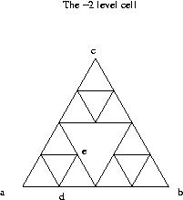
In the picture to the left, the largest cell drawn (the whole picture) is a level -2 cell, and a-2=-6, a-1=6, and a0=2. The formulas are as follows: f(d)=-f(a)/3+f(c)/3, and f(e)=-5f(a)/6+f(b)/6+f(c)/6. This was obtained just using linear algebra.