This revision makes it much easier to implement and explain some variant models.
The translation from TKF model to Needleman-Wunsch or  Smith-Waterman is
obvious from LMSH.  In the language of N-W, we can turn off gap penalties for
either leading or trailing gaps.  We can search for best aligned substrings.  Everything
is neatly expressed in terms of probabilities.   We can also find the probability of any
point in one sequence aligning opposite any point in a second sequence in the context
of an alignment process starting and ending anywhere within the observed sequences.

Note: I am not optimizing the parameters, e.g. time, substitution rate, death rate for
these models.  These are other features available with the TKF model which are
independent of the example shown below.

I concatenated three roughly 300 base subsequences from Species A and the
homologous subsequences from Species B, but in a different order.

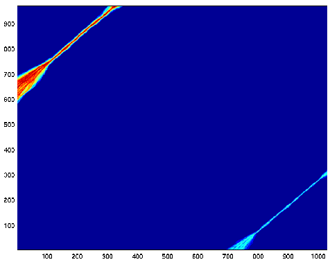
Here is the alignment picture for the TKF model, trailing gap penalty off:

Hooray!  The middle section aligns pretty well.  The start seems not so bad, but only because
we have gap costs at the beginning.

Let's turn off the leading gap penalty:

The exact start of the alignment is not perfectly clear.  We see that the first third of sequence
A aligns well with the last third of sequence B, and the last third of A aligns well with the first
of B, but the signal is not as strong.  The middle thirds disappeared in a sea of low probability.
There probably is a ridge in the middle, but getting there requires paying for two huge gaps.

Let's allow the alignment process to start and end anywhere.  We normalize all the alignment
data by the probability that we observed sequences A and B independently.

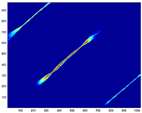
Now we can see all three segments at the same time.  When the trailing gaps are free, there
are also bright lines along the top and right edges from the ends of the well-aligned
subsequences.  These were so thin, that they got covered by the black border around the plot.

The different colors of the three bands indicates the relative strength of the three subalignments.
The strengths are dominated by the lengths.