Knot theory
II. Fundamental concepts of knot theory
Section1. Elementary knot moves
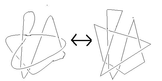
In the last lesson, we have learned the intuitive concept of equivalence of knots. In this section, let us formulate our intuitions mathematically. First, we can consider a knot to be polygonal in form, see fig.9. In this section, we think of a knot as being composed of a finite number of edges.
fig.9. These two knots are equivalent. So we are free to assume that all knots are composed of a finite number of edges.
For the sake of a precise mathematical interpretation of a knot, it is readily obvious that we can make alterations to the shape of a knot. For example, it is possible to replace an edge, AB, in space of a knot K by two new edges AC, CB. We can also perform the converse replacement. Such replacements are called elementary knot moves. Mathematically speaking, we shall now precisely define the possible moves/replacements.
Definition 2.1 On a given knot K, we may perform the following four operations.
(1) We may divide an edge, AB, in space of K into two edges, AC, CB, by placing a point C on the edge AB, see fig. 10
(1)' [The converse of (1)] If AC and CB are two adjacent edges of K such that if C is erased, AB becomes a straight line, then we may remove the point C, see fig. 10.
(2) Suppose C is a point in space that does not lie on K. If the triangle ABC, formed by AB and C , does not intersect K, with the exception of the edge AB, then we may remove AB and add the two edges AC and CB. See fig. 11.
(2)' [The converse of (2)] If there exists in space a triangle ABC that contain two adjacent edges AC and CB of K, and this triangle does not intersect K, except at the edges AC and CB, then we may delete the two edges AC, CB, and add the edge AC, see fig. 11.
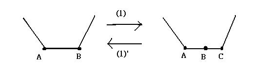
fig.10
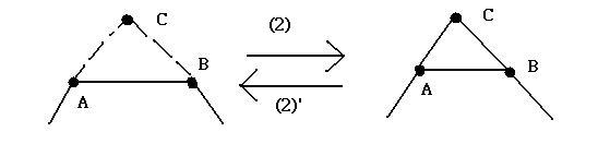
fig. 11
These four operations (1), (1)', (2), (2)' are called the elementary knot moves. [However, since (1), (1)' are not ''moves'' in the usual understanding of this word, often only (2), (2)' are referred to as elementary knot moves].
A knot is not perceptively changed if we apply only one elementary knot move. However, if we repeat the process at different places, several times, then the resultant knot seems to be a completely different knot. For example, let us look at the two knots P, Q in fig. 12, as we have seen in the last lesson, P is a trefoil knot. What about Q?
fig. 12.
Knots that can be changed from one to the other by applying the elementary knot move are said to be equivalent. From now on, we are going to use this as our definition of equivalence of knots:
Definition 2.2 A knot K is said to be equivalent to a knot K' if we can obtain K' from K by applying the elementary knot moves a finite number of times. We shall use the notation K~K' to denote the equivalence between the two knots K, K'. In knot theory, equivalent knots are treated without distinction, we shall consider them to be the same knot.
Exercise 2.1 Show that P, Q are equivalent by manipulations using your hands.
A knot has a closed curve so we can assign an orientation to the curve. As is the custom, we shall denote the orientation of a knot by an arrow on the curve. It is immediately obvious that any knot has two possible orientations, see fig. 13.
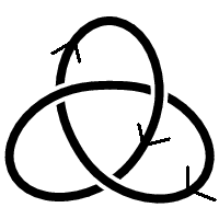
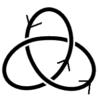
fig. 13 Trefoil knots with two orientations.
If two oriented knots , K, K' can be altered with respect to each other by means of oriented elementary knot moves, see fig. 14, then we say K and K' are equivalent with orientation, and write K=K'
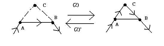
fig. 14 Oriented elementary knot moves with respect to (2),(2)' in definition 2.1
Two knots that are equivalent without an orientation assigned are not necessarily equivalent with orientation when we assign an orientation to the knots. The two knots in fig. 13 are certainly equivalent without an orientation assigned. However, it is not immediately obvious whether they are equivalent with orientations.
Section2. Links
So far we have only looked at a rather specific, but interesting in its own right, set, namely, knots. In this section we shall look at a generalization of this set, i.e. what happens when we ''link'' a number of knots together.
Definition 2.3 A link is a finite, ordered collection of knots that do not intersect each other. Each knot in this link is said to be a component of the link.
Definition 2.4 Two links L,L' are called equivalent if the following two conditions hold:
(1) m=n, that is, L,L' each have the same number of components.
(2) We can change L into L' by performing the elementary knot moves a finite number of times.
Example Corresponding to the trivial knot, the following fig.15 is called the trivial n-component link, which consists of n disjoint trivial knots:
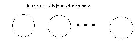
fig. 15
Exercise 2.2 Show that the following two links in fig.16 are equivalent. This link is called Whitehead link.
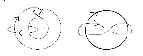
fig. 16
Exercise 2.3 Show that the following two links in fig. 17 are equivalent. This link is called the Borromean rings.
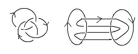
fig. 17
Section3. Operations on knots (A): Knot decomposition
In the next section, we define a sum/product operation on the set that comprises all knots. The sum there is conceptually the same as what you have been learning since primary school. But, instead of summing up two integers, we are going to add two knots together. Therefore, we shall look into how we can obtain a single knot from two knots, called the sum (or connected sum) of these two knots. However, since a detailed explanation of this operation is way too complicated, we shall delay a rigorous explanation a bit later until the next section. To get an insight into this approach, we shall first concentrate on the reverse operation, that is, we shall decompose a knot (or link) into two simpler knots. And it is exactly the content of this section.
Assume that you are holding a random knot in your hands (as usual), we try to decompose the knots into two disjoint knots. Physically speaking, the first thing we can try is to cut the knot (a closed string) into two parts. Then, we now have two disjoint but open strings. Now we can glue the two open ends of each knot together to get two disjoint knots. See fig. 18
.PNG)
.PNG)
fig. 18 Knot K is decomposed into K1 and K2, by cutting the edges through points A and B, then we join the two open ends together, for K1 and K2.
Notice that the choice of line joining A and B for each knot is arbitrary because if we connect A to B by means of some other simple polygonal line, we shall at once again decompose K into two knots say K1', K2'. It is reasonably straightforward to see that K1, K1', and K2,K2' are equivalent ( since we are able to apply elementary knot moves to the lines we are talking about)
If one of the two disjoint knots after decomposition id trivial, then strictly speaking, this is not a 'true' decomposition'. (Digression: At this point, try to think of the case that when you are factorizing an integer. To have a 'true' or 'effective' factorization, we want to have p<a, q<a in the factorization a=pq. So factorization like 6=6 x 1 is known as non-effective and we want to exclude such factorizations by naming them as trivial factorizations. That is why prime factorization is so effective and prime numbers enjoy primitive roles in the theory of numbers since prime numbers form the building blocks of the set of integers, with the product operation. Now we are facing a similar task here, we want to have a 'true/effective' decomposition on the set of knots, so we say that if one of the two disjoint knots after decomposition is trivial, then it is not a 'true' decomposition) For such a 'non-effective' ('not true') decomposition, see fig.19 below. Notice that K2 is a trivial knot, K and K1 are equivalent. So we do not think of K as being decomposed into simpler knot
.PNG)
.PNG)
fig. 19. K2 is a trivial knot and notice that K and K1 are equivalent.
When a true decomposition cannot be found for K, we say that K is a prime knot. In a sense, this is equivalent to how we define prime number. i.e. a natural number that cannot be decomposed into the product of two natural numbers, neither of which is 1.
From the above discussion, a knot K is either a prime knot or can be decomposed into at least two non-trivial knots. These two non-trivial knots are either themselves prime knots, or we may, again, decompose one or the other, or both of them, into non-trivial knots. We continue this process for the subsequent non-prime knots. You will be heartened to know that this process does not continue to infinity. In fact, not only is the process finite, but it also leads to a unique decomposition of a knot into prime knots. Succinctly this is expressed in the following theorem:
Theorem 2.1 (The existence and uniqueness of a decomposition of knots)
(1) (existence) Any knot can be decomposed into a finite number of prime knots.
(2) (uniqueness) This decomposition, excluding the order, is unique. That is to say, suppose we can decompose K in two ways: K1,K2,...,Km and K1',K2',...,Km'. Then n=m, and furthermore, if we suitably choose the subscript numbering of K1,K2,...,Km, then K1~K1', K2~K2',..., Km~Km'.
A proof of this theorem can be found on Schubert [Sc]. Notice that the above theorem also holds in the corresponding case of links.
Section4. Operations on knots (B): Sum of knots
Let us now think about the composition that brings about the converse of the above decomposition of knots. Essentially what we are looking for is the sum of two knots. First, however, let us explain why this ''sum'' is a touch more troublesome than the process of decomposition. For example, if we take two links it is not at all clear which component of these links we need to combine, so that we obtain a single link that is their sum. Even in the case of knots, there is also a hurdle to overcome. If we reverse the orientation on a knot, we know that it is not necessarily equivalent with orientation, to the knot with the original orientation. Therefore, when we combine two knots their orientations become important.
We shall show how to overcome the hurdle for two oriented knots. Suppose P is a point on an (oriented) knot K in space, we may think of P as the centre of a ball B, with a very small radius, that possesses the following two properties:
(1) K intersects (at right angles) exactly two points on the surface of the boundary sphere of the ball B
(2) In the interior of B, we have a 'trivial tangle' (or an unknotted tangle). See the following fig. 20:
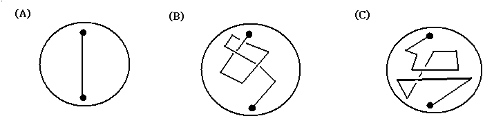
Fig. 20. (A) is a trivial (unknotted) tangle obviously. (C) is a trivial tangle as well, after slowing moving the string connecting the upper end and lower end. But (B) is NOT a trivial tangle since no matter how you move the string around, you are not able to get back the picture the same as (A)
In order to join (sum) two knots, the first step is to choose a point possessing the above two properties for each knot. Since we are able to have such a ball, like the one in (2), with this point as the centre for each knot, it just means that now we have two extreme points, the upper end point and the lower end point for these two balls, corresponding to each knot. Now, we can join the two upper end points together, similarly for the two lower end points. At this point, we obtain a new, single, oriented knot in our space. And we call the knot that is formed in the above process the connected sum of the two disjoint knots. We denote such a sum as K1*K2, where K1, K2 are the two disjoint knots that are joined together by the above process. For an example, see fig. 21
.PNG)
.PNG)
fig. 21. To join K1 and K2, we choose two balls, B1(left) for K1, B2(right) K2 in the left picture. Notice that these two balls with the corners inside as origins satisfy the two conditions above. Then, we join the upper end point with the upper end point for K1 and K2. Similarly, do the same thing for the lower end points of the two spheres. Eventually, we get the right picture. The two oriented red lines corresponds to the added lines in our joining process. Furthermore, it is now visibly clear that the knot in the right picture is a new, single, oriented knot, call it K. Mathematically, we denote it by K=K1*K2
Notice that this K1*K2 is independent of the two points that were originally chosen in each knot in the first step of the above process, as long as these two points satisfy the above two conditions. We can therefore say that K1*K2 is uniquely determined by K1 and K2.
From the definition of the connected sum of knots, the next theorem follows immediately (Recall: K1=K2 means that K1 is equivalent to K2 with orientation)
Theorem 2.2 The sum of two knots is commutative, that is,
K1*K2=K2*K1.
Also the associative law holds, that is,
(K1*K2)*K3=K1*(K2*K3)
Exercise 2.4 Instead of manipulations by hands, by using Theorem 2.1 and Theorem 2.2, show that the two knots below in fig. 22 are equivalent.
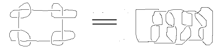
fig. 22
Exercise 2.5 Again, by Theorem 2.1 and Theorem 2.2, show that the two knots below in fig. 23 are NOT equivalent
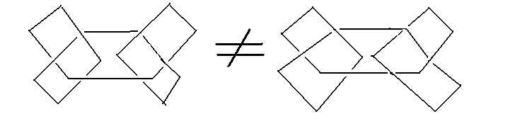
fig. 23
Recall: In the first lesson, we said that it is practically not feasible to determine whether two random knots are not equivalent. An important point here is that: To show that two knots are equivalent, we just need to manipulate the knots by hands. However, to show that two knots are not equivalent is a far more annoying task, since there are infinitely many number of ways to manipulate the knots. You can not say that ' These two knots are not equivalent because I am not able to solve it by pure physical manipulations'. The reason is: No matter how many times you have tried by your hands, there are still many more unpredictable ways to manipulate the knots in our space. So it is NOT A MATHEMATICAL PROOF at all! At this point, it is pretty clear that more mathematical tools are required to answer this problem. Now, by looking at Exercise 2.5, we experience, for the first time in our lessons, that abstract (is it really abstract up to this point?) mathematics plays its role in solving this problem effectively. More concretely speaking, we first have theorem 2.1, theorem 2.2 in our hands, then we go on to solve our problems, like Exercise 2.5, by applying the correct mathematical tools.