Knot theory
V. Knot invariants: Classical theory (continued) and Jones polynomial
In the last lesson, we have seen three important knot invariants: the minimum number of crossing points, the minimum bridge number and the minimum unknotting number. Here, we are going to see one more classical invariant in section 1-----the linking number, then we will move on to an entirely new type of knot invariant----Jones polynomial, in the remaining sections.
Section1. The linking number
Recall the orientation of a knot (or a link). Notice that the knot (or link) invariant we have discussed so far have all been independent of the assigned orientation of the knot. In this section we shall define look at an invariant which depends on the orientation.
First, let's assign either +1, -1 to each crossing point of a regular diagram of an oriented knot or link.
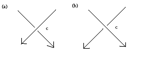
Definition 5.1 At a crossing point, c, of an oriented regular diagram, as shown in fig.40, we have two possible configurations. In case (a), we assign sign(c)=+1 to the crossing point, while in case (b) we assign sign(c)=-1. The crossing point in (a) is said to be positive, while that in (b) is said to be negative.
fig. 40
Suppose now that D is an oriented regular diagram of a 2-component link L={ K1, K2 }. Further, suppose that the crossing points of D at which the projection of K1 and K2 intersect are
![]()
(We ignore the crossing points of the projections of K1, and K2, which are self intersections of the knot component) . Then,
![]()
is called the linking number of K1 and K2, which we shall denote by lk(K1,K2). Indeed, it is an invariant of the link L, for a proof, see K. Murasugi [Mu]:
Theorem 5.1 The linking number lk(K1,K2) is an invariant for L
That is to say, if we consider another oriented regular diagram, D' of L, then the value of the linking number is the same as for D. Therefore, we shall call this number the linking number of L, and denote it by lk(L). Further, the linking number is independent of the order of K1 and K2, i.e.
![]()
Exercise 5.1 Let us calculate the linking number of the links L, L' in fig. 41(a) and fig. 41(b) respectively. By considering the four crossing points in fig.41(a), fig.41(b). Show that for fig. 41(a),
![]()
Likewise, for fig. 41(b),
![]()
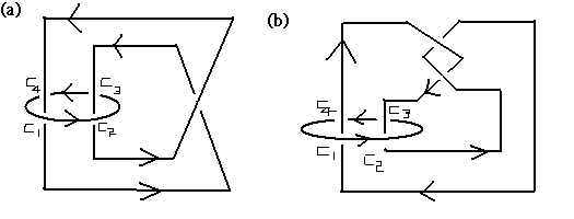
fig. 41
Exercise 5.2 By using Jordan curve theorem, show that the linking number is always an integer.
Exercise 5.3 Suppose that we reverse the orientation of K2, which we will denote by -K2, show that
![]()
Therefore, by exercise 5.3, the linking number is an invariant that depends on the orientations of the knot components.
Suppose now that L is a link with n components, call them
![]()
With regard to the i-th and j-th (i<j) components, we may define an extension of the above linking number (by ignoring all the other components except the i-th component and the j-th component) :
![]()
This approach will give us, in all (n(n-1))/2 ( do you know why? ) linking numbers and their sum:
![]()
It is called the total linking number of L.
Exercise 5.4 By applying theorem 5.1 and using mathematical induction, show that the total linking number is an invariant for L
Exercise 5.5 Calculate the total linking number of the following two links in fig. 42.
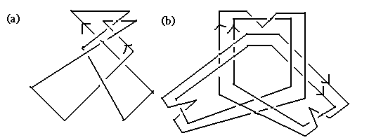
fig. 42
Section2. The Jones polynomial
In 1984, after nearly half a century in which the main focus in knot theory was the knot invariants derived from the geometry of knot, that is, the knot invariants which had been well-studied were based on the shape of the knot, V. Jones announced the discovery of a new invariant. Instead of further propagating pure theory in knot theory, this new invariant and its subsequent offshoots unlocked connections to various applicable disciplines, some of which we will briefly discuss in the later lessons. Originally, Jones defined this invariant based on deep techniques in advanced mathematics. Soon after his discovery, it became clear that this polynomial could be constructed using methods in other disciplines. In this section, our intention is to study the new invariants from the point of view of knot theory, explaining several of their fundamental properties.
Definition 5.2 Suppose K is an oriented knot (or link) and D is a (oriented) regular diagram for K. Then the Jones polynomial of K can be defined uniquely from the following two axioms. The polynomial itself is a Laurent polynomial in the square root of t, that is, it may have terms in which the square root of t has a negative exponent. This polynomial is a knot invariant for K.
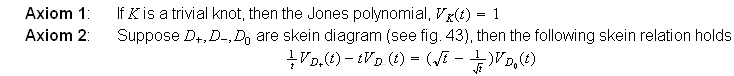
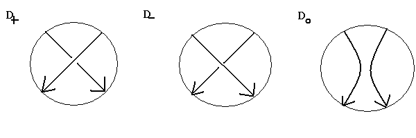
fig. 43
As we have talked about at the beginning of this section, the definition of the Jones polynomial is entirely different from all the knot invariants we have seen before. In order not to obscure the big picture, we should first discuss the algorithm to compute the Jones polynomial and its fundamental properties.
Indeed, the Jones polynomial can be applied to a link as well, let O(u) be the trivial u-component link. Then we have the following theorem:
Theorem 5.2
![]()
Proof: The proof will be by induction on u. If u=1, then it is just the Axiom 1. So let us assume our inductive hypothesis in the following:
![]()
If we consider the skein diagram (fig. 44)
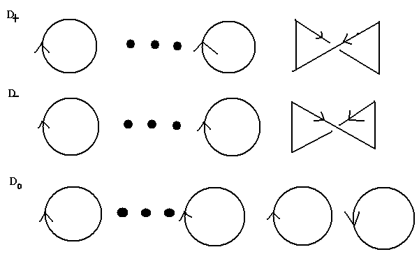
fig. 44 The top picture has (u-2) copies of circles, so does the middle picture. But the picture at the bottom has u circles. Notice that the top oriented regular diagram is equivalent to the regular diagram of O(u-1), so does the middle one.
then we have :
![]()
By the inductive hypothesis and skein relation in Axiom 2 in the definition of the Jones polynomial, we have:
![]()
The left side of this equation is :
![]()
Hence the theorem follows. (The end of the proof)
The most effective way to compute the Jones polynomial is to write down the skein tree diagram for the knot. Before doing it, by muddling around with the equality stated in the Axiom 2 in the definition of the Jones polynomial, we have the following two inequalities :
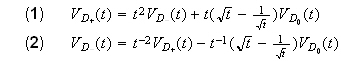
Exercise 5.6 By using the equality stated in Axiom 2, prove the above two inequalities.
From now on, let
![]()
then from (1), (2), we have:
![]()
Let's look at the following skein tree diagram of a oriented trefoil knot :
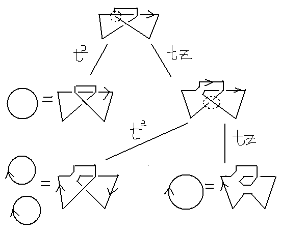
fig. 45. The first row consists of just the original trefoil knot. Here, we focus on the dotted circle on one of the crossing point. (The aim here is to apply the skein relation in the Axiom 2.) From the top row to the second row, we have applied equation (3) at the crossing point in the dotted circle. In the second row, the left knot is equivalent to a trivial one so we do need to apply the skein relation again. But for the second one, which is still knotted, we apply equation (3) once more at the point in the dotted circle.
Exercise 5.7 We have drawn the skein tree diagram for the oriented trefoil knot. Show, by using fig.45 and equation (3) and theorem 5.2, that:
![]()
Exercise 5.8 Using the same method as the previous exercise, by constructing the skein tree diagram yourself, show that, for the Whitehead link (fig. 46), we have the below Jones polynomial of it.
![]()
fig. 46. Whitehead link
It is, at first, intriguing to see that such a weird-looking definition of a ' polynomial ' turns out to be a powerful knot (or link) invariant. But it can be proved that it is so. The proof of it will bring us beyond the scope of these lessons, without significantly illuminating our future discussions so we decide to skip it here. For a proof of it, see Lickorish[Li].
Although the Jones polynomail is a powerful invariant, it is not a complete invariant. That is to say, there exists an infinite number of non-equivalent knots that have the same Jones polynomial. See [Kan] for an example. In his paper, he showed that the Jones polynomials of the two knots are the same but they are inequivalent. Furthermore, it is still an open problem whether the Jones polynomial classifies the trivial knot, that is, if, for a given knot, its Jones polynomial is 1, does it necessarily imply that it is a trivial knot?