With this explanation, certain examples, such as numbers in the newspaper, following this distribution seem to make more sense. To understand how to get the exact probability try the following Exercise.
Exercise 2: calculate the time spent from 10 to 20. Using properties of logarithm, what can you conclude?
From this exercise, you can kind of see the fraction of time spent from 1 to 2, 10-20, 100-200, ... versus the total time is just the fraction of time spent from 1 to 2 versus 1 to 10. Using properties of log, the answer is log 2 =0.301.... This is exactly the one appearing in the above graph.With this calculation we obtain the log distribution: probability that the leading digit is d equals log(d+1)-log(d)=log (1+1/d).
Definition: A sequence of numbers  is Benford if the leading digits approaching the log distribution in the limit as n approches infinity.
Multiplicative (Geometric): It turns out that lots of phenomena that are multiplicative in nature can be shown to satisfy Benford's law. The way it is proved is similar to exponential growth. From log ab = log a + log b, we can reduce multiplicative processes to linear ones, which is usually easier. For example, the stock market can be modeled by multiplying it by 2 and 1/2 with probability .5 and .5 , respectively, every year (where the values given are arbitrary and certainly inaccurate). If we take log, this becomes adding 1 and -1 with probability .5 and .5, which is like flipping a coin and trying to figure out the total number of heads after some time (the latter is called random walk and can be modeled by a bell-shaped curve by the Central Limit Theorem; the former is called geometric Brownian motion (illustrated below) and satisfies Benford's law)
To give a definition of scale-invariance, we start with a sequence  with the probability that a number from the sequence has leading digit less than d denoted by D(d), then this probability will be the same as that of the sequence
  , for any c>0.
Similarly we can change the number system we use: instead of base 10, we use base 8. We hope this will again give us log is the only distribution that work (this won't work though because the sequence {1, 1, 1, ...} is the same no matter what base we are in. That means the distribution with 1 being 1 and everything else 0 will screw things up. But that's the only problem.)
