Numb3rs 219: Dark Matter

In this episode Charlie uses a support vector classifier in an attempt to identify the remaining school shooter. A support vector classifier, or rather support vector machine (SVM), as it's more commonly known, is a method for classifying objects described by a given set of properties into groups. While this definition may leave you underwhelmed, keep in mind that the problem of classification lies at the heart of intelligent behavior. It takes you a split of looking at a photo to recognize a tree, a car, a friend, but for a computer, image classification is a very hard task indeed. On the flip side of the coin, it may take an FBI agent weeks or months to pour over records and decide which individuals most closely fit the profile of a school shooter, but a well designed SVM may do so in seconds or minutes. Making SVMs do things like image or voice recognition quickly and accurately is a currently hot research topics in artificial intelligence. So how do SVMs work? Let's find out!

Vectors, Matrices, and the Stuff They Do

Before we can explore SVMs, we need some understanding of vectors and matrices. (Actually, if you only want to understand the introduction to SVMs contained in the following section, you only need to know what vectors are and what a dot procuct is. If you wish to learn more about SVMs, or are interested in learning a fundamental tool of mathematics, you ought to master the material on matrices below.)
A vector is simply an ordered list of numbers, called coordinates. For instance, (2, 5) is a 2-vector, i.e. a vector of dimension 2, while (-3, 1.4, 5) is a 3-vector. Usually vectors are represented as arrows in the Euclidean space of the corresponding dimension: arrows starting at the origin and ending at the point corresponding to the coordinates, as in the picture to the right. At other times vectors are represented simply by the point corresponding to their coordinates, to avoid cluttering the picture. Vectors of the same dimension can be added and subtracted, simply by adding and subtracting the pairs of corresponding coordinates: (2, 5)+(-4, 3.3)=(-2, 8.3). Vectors can also be multiplied by a number, by multiplying each coordinate by that number: -4*(2, 5)=(-8, -20).

Activity 1: To the right you see the geometric representation of vector addition. What geometric figure do the blue vector lines and dotted lines produce? Draw a similar diagram for vector subtraction, say for (5, 1)-(1, 2)=(4, -1) and find the corresponding parallelogram.

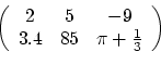
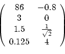
A matrix is an array of vectors stacked on top of each other. One way to think of it is as a vector of vectors. The first matrix below is a 2x3 matrix (2 rows, 3 columns), while the second is 4x2.

When multiplying a matrix by a number, you simply multiply each entry by that number, just like for vectors. Two matrices of the same size can be added together by adding the corresponding entries, just like for vectors.

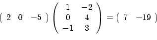
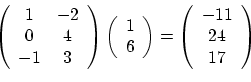
Multiplying a matrix by a vector is the same as multiplying a matrix by another matrix, with one of them having only one row or column. Now we have to differentiate between column vectors, which are matrices with one column, and row vectors, which are matrices with one row. Thus a 3x2 matrix A can be multiplied by a row 3-vector (a 1x3 matrix) as VA, resulting in a row 2-vector, or by a column 2-vector (a 2x1 matrix) on the right, as AV, resulting in a column 3-vector (see example below).

Usually vector means column vector, but not always, so pay attention to the context.

Now that you've done the activities above, we have a new way of thinking of matrices. You can think of a function of one variable, say f(x)=2x+5, as a machine into which you feed a number, x, and get back a different number 2x+5. For a two variable function, f(x,y)=x+y say, you feed in two numbers, x and y, to get back one, x+y. With matrices things get more interesting: you feed in a vector and get back a vector!

Support Vector Machines

Suppose you want to teach a computer to differentiate between a handwritten digit 1 and a handwritten 0. First you gather a sample of say 50 handwritten ones and 50 handwritten zeroes, from different people, and scan them to produce digital images, each measuring 100 by 100 pixels. Every pixel has a color, which is given by a non-negative integer. Thus you can represent each scanned digit image as a 10000-vector: each pixel corresponding to one vector coordinate and that pixel's color corresponding to the numeric value of the coordinate. For instance, if we have only 256 colors, a "picture" consisting of 4 pixels can be represented by a 4-vector, each coordinate of which can take on values from 0 to 255. The problem is then to find a rule using which a computer, given a new 10000-vector, can decide whether the vector represents a picture of a 0 or a 1.

Activity 1: Let's make life easier for ourselves and examine the case of 2-vectors, which we will draw as points on the Cartesian plane (we'll have a whole bunch of them, so drawing arrows is impractical).

1. Suppose you ask 40 random participants in this year's Boston Marathon their height and time spent training per week. You then divide them into two groups, those that completed the marathon and those that did not and plot this data as in Figure 1 below. Based on this data, if I give you the height and weekly training time of another runner, could you tell whether the runner is likely to complete next year's marathon? How confident would you be in this prediction? What if I only tell you the runner's height? How about if you only know the weekly training time?
2. How about the data vectors in Figure 2? Given a new vector (a new data point) how confident will you be in guessing to which group it belongs? What if you simply know that the x component of a new vector, without knowing the y component?
3. How does the data in figures 3 and 4 differ? In what case is classification easier?

As you've seen in the activities above, in some cases the classification problem is easier, in others harder or impossible. The basic idea behind SVMs is to use lines for 2-vector data and planes for 3-vector data (in general hyperplanes) to divide the space in which the vectors live into two "halves": a half in which only vectors from one group are located and a half in which vectors from the other group lie. New vectors are then classified depending on which half they lie in. For 2-vectors and lines, this is sometimes possible, as in the case of Figure 2 above, and sometimes not, as in the case of Figure 1. That is, you can't separate the two vector groups in Figure 1 by a line while you can in Figure 2. In the case where you can separate data groups by a line, how do you find the best line that separates the data? Good question! Let's proceed to activity 2.

Activity 2:

1. Two vectors v and w are called orthogonal when their dot product v·w is zero. Find a vector orthogonal to (5,3). Find a different one. Draw all three vectors.
2. One way to define a line through the origin on the Cartesian plane is by specifying a normal vector v, i.e. a vector to which all points on the line are orthogonal (see right). What vector is normal to the x-axis? To the x=y line?
3. We can use the above idea to define a line through the original by an equation such as (x,y)·(-3,-2)=0. Convert this equation to the usual slope-intercept form for an equation of a line. Write a different dot product equation for this line (i.e. use a vector different from (-3,-2), and again convert it to slope-intercept form.
4. Now we know how to write lines through the origin in terms of normal vectors. What about lines not passing through the origin? The key observation is that such lines are simply lines through the origins shifted over in some direction. Draw the line corresponding to (x,y)·(3,4)+5=0. What's the dot product equation of the line y=7x+2?
5. Where is the region (x,y)·(-1,2)+4<0 located? How about (x,y)·(0,1)+10>0?

The distance from a vector v to a line given by (x,y)·w+c=0, where w is a 2-vector and c a number, is defined as the shortest distance between v and any point on the line and is equal to . Note that in the numerator |v·w+c| means absolute value, while in the denominator ||w|| means the length of the vector w. Suppose our initial data is given by vectors v₁, v₂, ... ,v_k, each belonging to groups 1 or 2. Using the ideas above, we can think of finding the best separating line by finding a 2-vector w and a number c such that

• the line (x,y)·w+c=0 separates the two groups of vectors
• the distance from the line to the closest vector in group 1, call it d₁, plus the distance to the closest vector of group 2, call it d₂, is the largest possible

All right, so now we know the idea behind SVMs: find a separating line (or hyperplane, in the general n-vector data case) and classify new vectors based on which side of the line they fall on. What about a situation similar to Figure 1 in Activity 1, where it's impossible to separate the data with a line? There are a few approaches. The most simple one is to separate the data to the best possible degree. That is, allow vectors in both groups to be located on both sides of the "separating" line, but minimize the resulting error: find a line so as to minimize the distances to the vectors located on the wrong side (see illustration to the right). This method, however, would give terrible results in cases like that of Figure 3, where the data is "separable" but not by a line! This is where the real magic happens: what we do is map our data to a higher dimensional space in such a way that in the new space we can separate it with a plane. For the data in Figure 3 for instance, one way to do this is to use a map like f(x,y)=x²+y². See the illustration below.

When the initial data vectors are easy to visualize, such as in the case of the above examples of vectors in the plane, it's often easy to find a map to a higher dimensional space where the data can be separated. However, in real world applications, such as handwriting recognition which I described earlier, it's not feasible to "look" at 1000-vectors and "see" the suitable map. Thus much of the current research in SVMs focuses on finding good generic maps, often to very high dimensional spaces (or even infinitely dimensional), which produce good results for whole categories of initial data, like the category of written characters or the category of speech recognition.