Numb3rs 101: Pilot

In this episode, a serial murder-rapist has made numerous attacks in the Los Angeles area.  Making some seemingly harmless basic assumptions, Charlie builds a statistical model of the attacker's behavior which helps the FBI stop the murders.

What does practical mean?

A model of the attacker's behavior could be a number of different things.  Don and the FBI want to know where the next attack will be.  Charlie points out that this might be the incorrect approach to the problem by making an analogy to a sprinkler.  He proposes that finding the sprinkler would be easier than deducing the location of the next point where a drop will hit.  In many ways, Charlie is probably correct.  We can probably assume that the killer has an apartment where he or she spends quite a bit of time.  If we can find the most likely neighborhood where the attacker resides, it should be easier on FBI resources than sending a dozen agents to patrol several neighborhoods searching for an attack in progress.  A second reason, going back to the analogy of the sprinkler, is that the physics of finding the next sprinkler drop are quite complicated; by this, Charlie means that regardless of how many drops we've seen hit the ground, the area where we should look for the next drop to hit will be quite large.  In the best possible model, more data should provide significantly better deductions.  Since the sprinkler is stationary, however, the seeming randomness of the action of physics on each droplet will affect Charlie's model less and less as the number of droplets are observed.

We will define a model of the attacker's behavior to be a function p(x) from the addresses in Los Angeles to the unit interval (the interval [0,1]).  That is to say that if x is a location in Los Angeles, then p(x) is a number between 0 and 1.  Not just any function will do, however.  We require the function p(x) to have the following property: when we sum the values p(x) over all addresses, the result is 1.  We then call p(x) the probability that x is the killer's address.  Where p(x) is higher, the assailant is more likely to reside.

After thinking about the problem briefly, we realize that we have our hands full: there are infinitely many models to choose from.  We somehow need to find the right one.  However, we don't even have a concept of what right means.  In laymen's terms, we need the model to "fit the data."  How do we quantify this common notion so that we may make mathematical deductions?  Charlie makes a point that when a person tries to make a bunch of points on a plane appear randomly distributed, the result is that the points adjacent to any given point x are all approximately the same distance away from x.  Charlie uses this information to produce his model.  As one can see from the map Charlie brings to the FBI, the "hot spot" - the most likely area where the perpetrator lives - which Charlie computes is in what we might imagine is the "center" of the attacks.

Unfortunately, Charlie's model fails.  The FBI gets DNA samples from every resident of the neighborhood Charlie says they should check, but none of the DNA matches the perpetrator's.  So, Charlie has to ask himself if the model he made was good.  He sees one data point which appears anomalous.  However, any model with the properties we outlined above shouldn't be affected too much by a single data point.  Indeed, after fixing the error, Charlie's new model has a smaller hot zone which lies completely within the one the FBI already checked.  He is stunned by the realization that his model is bad.

 Eventually, Charlie realizes that he has made a classic error.  It is sometimes quipped that the only difference between physicists and engineers is that physicists can be sloppy in their approximations.  A physicist wanting to produce a set of laws of physics which is as complete as possible will not choose the most complicated set of laws before trying out a simpler set first.  In the same way, Charlie chooses the mathematically practical approach by choosing the simplest possible solution to his problem by assuming there would be exactly one hot zone.  It is mathematically practical in the sense that solving this complicated problem is a lot easier with one hot zone than two.  Generally this is a good way to approach a problem; at worst one learns why the easy approach does not work which hopefully gives some clues as to what the more complicated approach should look like.  With two hot zones (one representing home and the other representing work), Charlie's model gives more accurate results: one hot zone is in the same neighborhood as before, the other is in an industrial area, and the hottest parts of the hot zones are quite small.  After making the arrest, Don notices that the perpetrator had moved from the original hot zone a few weeks ago, which is why the FBI hadn't found him in their original search.

How did Charlie produce his model?

Of all the possible models, how did Charlie find that specific one?  Not many clues are given in the episode as to what method he uses.  So, let's consider the following more tractable problem.  Suppose we have done the following experiment: we hung a spring from the ceiling and measured the lengths of the spring after attaching a weight.  After doing this for several different weights, we have collected a bunch of data.  After making a graph of weight versus change in length, we might notice that the points form almost a line (assuming the weights aren't too heavy).  This means that if the weight is W and the change in length is L, W=kL for some number k (this relationship is called Hooke's law after the British physicist born in the 1600s).  How do we compute k?  We could draw in a bunch of lines which seem to approximate our data well and pick the one which is the best.  This is called the linear regression problem.  But which one is the best?  There are many different concepts of that, and the simplest one isn't the one we generally use.

Let M denote the set of all lines through the origin.  M is our set of models.  Let S denote the set of points which we have computed experimentally.  Given any line W(L) in the set M and data point (x,y), compute the quantity , the vertical distance between the line W and the point (x,y).  Add up the quantities  for each point in S.  This gives us a mapping from the set of models to the non-negative real numbers.  Generally, a map from a set of functions (in this case, lines) to the real numbers is called a functional.  Denote our functional by A(W).  If we can find a line for which A(W) = 0, then our data points are all colinear.  This is generally not going to happen.  The next best thing would be to find a line W for which A(W) is as small as possible.  In this case, we say that such a line W minimizes A(W).

So now we must find a line which minimizes A(W).  When one wishes to minimize a quantity, one generally uses differential calculus.  Unfortunately, the absolute value function has no derivative at zero.  So, square the distance first!  Instead of adding up to create A(W), we add up .  This is called the method of least squares and is generally the accepted method of solving the linear regression problem.  To solve the problem requires a little calculus.  Wolfram's website has a relatively good explanation.

Notice that there was nothing special about the line here.  Any set of functions M and non-negative functional A(W) would have worked (although there will be technical problems if M and A are not chosen wisely, such as not being able to find a minimizing function inside our set M).  So we could have found the quadratic polynomial of best fit or the exponential of best fit in a similar fashion, although solving such a problem will no doubt be vastly more complicated.

This method is a general approach used by mathematicians in a variety of situations.  The difficulty is generally in proving the existence of a function which minimizes whichever functional we have decided to work with.  In physics, one often hears that objects take the path of least action or least energy.  That is to say that rather than solving a very complicated differential equation, we could solve a variational problem instead.  This method is so useful that it is basis of theoretical physics.

Random sequences?

Charlie makes a comment that to consciously construct a random sequence is impossible.  This is true in many ways.  As an example, consider the following property of sequences due to Khinchin.  Given any real number x we can find a continued fraction expansion

 

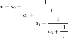
In fact, as long as x is irrational, the continued fraction expansion is unique.  Khinchin's Theorem says that

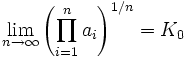
for almost every continued fraction.  Here almost every refers to a somewhat complicated notion from measure theory.  Luckily, in our case it means exactly what it sounds like.  What is interesting is that no one has been able to demonstrate a continued fraction which has the property given above.  So, truly, we are not very good at coming up with random sequences at all!