
A doctor finds new evidence that could exonerate a mob boss from the death penalty. Charlie and the team have only few hours to run down the evidence and make sure justice occurs.
In the beginning of the episode Charlie uses Gaussian filtering to clean up some documents that could serve as evidence in the case. Before we describe this image and signal process methodology, we need to understand a key operation in this process, namely convolution.
Convolution is an operation between two functions f and g that produces a new function denoted by f*g. This operation has some nice properties that resemble the ones satisfied by the usual pointwise multiplication of functions. Even though the physical and mathematical nature of these two operations is different, the two are related through the Fourier transform. In what follows, we will explicitly define the discrete convolution and clarify the claims stated above through an example.
Suppose that f and g are discrete functions that assign to any integer number n (i.e. n=...,-2,-1,0,1,2,...) the value f(n) and g(n), respectively. These functions could represent for instance temperatures at different points of an infinite rod where the position on the rod is codified by n, or (expected) average earth's population over the past and future years where the current year is represented by n=0. The convolution of f and g, denoted by f*g, is a function whose value at any integer n is given by the formula
Observe that for each integer number m, the corresponding term in the infinite sum above is f(m)g(n-m). Hence, the convolution corresponds to the sum of the values obtained after pointwise multiplication of f times a shifted and reversed version of g (see Tangent). Since most of the functions that represent some type of signal in the real world are finite we state a particular case of the definition above when f and g take the value zero for all n except possibly for n=0,1,...,N. In this case, f*g takes the value zero for all n except possibly for n=0,1,...,2N (to verify this fact use parts b) and c) of Activity 1 below) and for each of these n, f*g(n) is given by

Let's consider the following example. Suppose that f(n)=1 for n=0,1,2,3 and f(n)=0 otherwise, and g(n)=f(n) for all n. The figure below shows a graphical representation of these two functions and their convolution f*g.

In this particular case the pointwise multiplication of f and g is equal to f itself. Hence there is a clear difference between the pointwise product and the convolution of f and g. There exists however a fundamental relationship between these two operations that is stated in the Convolution Theorem.
Convolution Theorem: The Fourier Transform of the convolution of two functions is the pointwise product of their Fourier Transforms.
In the language of signal analysis this theorem states that when convoluting two functions their corresponding frequencies multiply. In order to gain a better understanding of the Convolution Theorem and to find out more about Fourier Analysis, we refer the reader to "A wavelet tour of signal processing" by Stephane Mallat.
We conclude by presenting some interesting properties of the convolution operation. Notice the resemblance to the ones satisfied by the usual multiplication of numbers. Let f,g and h be arbitrary functions then,
1) f*g=g*f (Commutative)
2) f*(g*h)=(f*g)*h (Associative).
3) f*(g+h)=f*g+f*h (Distributive law)
One can think of an image as a rectangular array of numbers, where each number represents the intensity at the corresponding pixel. If this array has m rows and n columns we say that the size of the image is mxn. Each row (resp. column) can be considered as a function f(k) on the integers that takes the corresponding values for k=0,1,...,n-1 (resp. k=0,1,...,m-1) and it is equal to zero otherwise. In image processing, Gaussian Filtering or Gaussian Blur describes the process of taking the convolution of these row and column functions with functions of the form
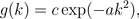
where c and a are appropriately chosen constants. These functions are known as Gaussian Functions and in this context are called Gaussian filters (see Tangent). The effect of this operation is a reduction of details on the image and hence a blur (the image on the right of the figure below is the blurred version of the image on the left). This occurs because the Gaussian Functions satisfy very particular properties that smooth out certain futures of the image, in particular its edges. Gaussian Functions are infinitely smooth and their smoothness is transmitted through the convolution.


To clean up the evidence, Charlie uses Inverse Gaussian Filtering. This process recovers the original image from its blurred version. In order to do so one can use the Convolution Theorem (see above) by taking the Inverse Fourier Transform of the Fourier Transform of the distorted image divided by the Fourier transform of the filter. This application highlights the importance of the Convolution Theorem in Image Processing. The methods and concepts described above extend the ones presented in Episode 3-19.