Numb3rs 519: Animal Rites
A disturbed student, tied to an animal rights group,
is implicated in the death of a researcher at CalSci. The arrestation
attempt of this lead suspect turns into a hostage
situation. In order to rescue the hostages and get into the student's
mind, Charlie and Amita investigate the student's work in
mathematics. They find his math to be highly creative but
formally incorrect. In some of the papers they discover an ecological
version of the Prisoner's dilemma (a concept already presented in Episode
110 and Episode
321), which reveals the suspect's immense appreciation for
animals.
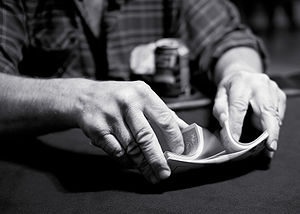
In
the beginning of the episode, while playing poker with Amita,
Liz and Nikki, Larry mentions a well-known result in the mathematics of
shuffling
cards discovered by mathematician and magician Persi
Diaconis at Stanford University.
"Actually, Nikki makes a
critical point. Persi Diaconis at Stanford proved a minimum
of five shuffles are required before a deck starts to become
random in the sense of variation distance described in Markov
chain mixing time, but seven shuffles are optimum."
Below, we will explain this
and other related results in more detail.
Riffle shuffle
Some people lift the cards up after a riffle in order to put the two
halves together.
Others place the halves flat on the table with their corners touching,
lifting the edges with their
thumbs while pushing the two halves together. A reason why
this is one of the preferred methods of shuffling is that the
cards are
rarely exposed during this shuffle.
The riffle
or dovetail
shuffle is the most commonly used method of shuffling cards. In this
shuffle the deck is cut in two halves, which are then interleaved or
riffled together (see Tangent). Gilbert
and Shannon in 1955 and independently Reeds in 1985 introduced a mathematical
model of this type of
shuffle. In
this probabilistic model, the probability
that exactly k
cards are cut off a deck with n
cards is C(n,k)/2n,
where C(n,k)
is the binomial
coefficient; i.e. the size of the cut off has a binomial
distribution with p=1/2.
The k
cards that have been cut are held in the left hand
and the remaining n-k
in the right hand. After the cut, the cards are
dropped from a given hand with probability proportional to the packet
size. Thus, if at some point there are c
cards on the left packet and d
cards have been already dropped on the table the probability that the
next card is dropped from the left is c/n-d.
Diaconis in
1988 found evidence showing that this mathematical
description is a reasonable approximation of the actual behavior of
human shufflers.
 There is a backwards description of the riffle shuffle that is helpful
for its mathematical analysis. In an
inverse riffle shuffle,
each card in a sorted deck goes to either the left or right packet with
probability 1/2. Then, the left packet is placed on top of the deck,
keeping the cards in the same relative order. It turns out that the
Gilbert-Shannon-Reeds model is equivalent to the inverse riffle shuffle
from the probabilistic point of view. To illustrate this fact we
present an example.
There is a backwards description of the riffle shuffle that is helpful
for its mathematical analysis. In an
inverse riffle shuffle,
each card in a sorted deck goes to either the left or right packet with
probability 1/2. Then, the left packet is placed on top of the deck,
keeping the cards in the same relative order. It turns out that the
Gilbert-Shannon-Reeds model is equivalent to the inverse riffle shuffle
from the probabilistic point of view. To illustrate this fact we
present an example.
Suppose that we have a deck consisting of only 4
cards with initial configuration A♠ 2♠ 3♠ 4♠. Let's calculate the
probability that after 1 forward riffle shuffle the new configuration
is A♠ 2♠ 4♠ 3♠. In this case 3 cards are cut from the top,
namely A♠ 2♠ 3♠. This happens with probability C(4,3)/24=1/4.
Then the first card, 3♠, is
dropped from the left packet and the second, 4♠, from the
right packet. This occurs with probability 3/4*1/3=1/4. Multiplying
these two probabilities out we conclude that under the
Gilbert-Shannon-Reeds model the probability of this configuration is 1/16.
Let's now calculate the probability that after one inverse
riffle shuffle we obtain the same configuration. In this case,
A♠ 2♠ 4♠ go to the left packet, while 3♠ goes to the
right packet. This occurs with probability 1/2*1/2*1/2*1/2=1/16.
The probabilities under the two models are the same. This fact can be
generalized to an arbitrary number of shuffles and the exact
probability of a given configuration will be given below.
First we highlight an important observation about the riffle
shuffle. Suppose that we
number our cards from 1
to n.
A riffle shuffle generates a permutation
of this n
numbers. If we denote this permutation by π,
in our example above
π(1)=1,
π(2)=2, π(3)=4 and π(4)=3,
i.e.
π(i) gives us the new position of the i-th
card.
A rising sequence of a permutation is a maximal consecutively
increasing sequence in the permutation. For instance, in our example
there are two rising sequences, namely
π(1)<π(2)<π(3)
and π(4).
If we had six cards and
π(1)=1,
π(2)=2, π(3)=4,
π(4)=3, π(5)=6
and π(6)=5,
there would be three rising sequences, namely
π(1)<π(2)<π(3), π(4)<π(5) and
π(6).
Rising sequences are the basis of a card trick called
Premo
by
Jordan.
In this trick the performer asks a spectator to riffle shuffle an
unshuffled deck of cards twice, then to give it a cut and insert the
top card into the pack. Give the pack a final cut and a final shuffle.
The performer spreads the deck on the table and after a careful
analysis
selects a card. The strategy to find the correct card is explained in
detail in Section 2 of Diaconis and Bayer's paper "
Trailing
the dovetail shuffle to its lair". The solution arises
mainly from the fact that (usually) each riffle shuffle duplicates the
number of rising sequences of the deck and inserting a card into the
deck increases this number by one.
It is easily seen that a permutation π of
any number of cards made by a riffle shuffle has exactly two rising
sequences, unless no shuffle is made whatsoever. Hence for instance the
permutation of 6 cards presented above cannot come from a riffle
shuffle. Conversely any permutation with 1 or 2 rising sequences can be
achieved by a riffle shuffle and this type of shuffle can be
characterized by this fact (see Tangent). It is not surprising then
that
the probability of a given configuration after an arbitrary number of
riffle shuffles can be given in terms of the number of rising
sequences. The following theorem was proven by Diaconis and Bayer in their
celebrated paper "Trailing
the dovetail shuffle to its lair" in 1992.
Theorem: If
n cards are shuffled
m times, then the chance that the deck is in arrangement π is
C(2m+n-r,n)/2nm,
where r is
the number of rising sequences in π.
- Activity 1
a) There are two ways to perfect riffle shuffle a deck of 2n
cards. Both
methods cut the
deck in half perfectly. The 'out shuffle' leaves the top card in the
same
position while the 'in shuffle'
moves it to the second position from top to bottom. These methods are
also known by the name of Faro shuffle. How many in (out) Faro shuffles
are needed
to return a deck with 4 cards to its initial configuration? How many
for a 52 cards deck? To find out more about the history of the perfect
shuffle we refer the reader
to Section 3 of Diaconis, Grahams and Kantor's 1983' paper
titled "The
mathematics of the perfect shuffle".
b) By using Bayer and Diaconis' theorem recalculate the probabilities
in the example above. Furthermore, observe
that the probabilities of obtaining any configuration after one shuffle
are all the same.
c) Suppose that a deck of 8
cards has initial configuration
A♠ 2♠ 3♠ 4♠ A♥ 2♥ 3♥ 4♥.
Calculate the probability that
after 2 riffle shuffles the new configuration is
3♠ 3♥ 4♥ A♠ 4♠
2♠ A♥ 2♥
Randomization
A deck of n
cards is perfectly random if the probability of any of the n!=1*2...*n
possible orders of the deck is the same, i.e. if the distribution of
all possible orders is uniform.
One possible way of measuring how random is a deck of cards after m
shuffles is by measuring the total
variation distance between the distribution of
the permutations after the m
shuffles and the distribution in a perfectly random
deck. Below we explain the definition of the total variation distance
in
our context. We also present Persi Diaconis and Dave Bayer's famous
result on the
number of riffle shuffles needed to achieve a good level of randomness
in a deck of cards.
The total
variation distance between two probabilities P
and Q
over the set of permutations is
defined as
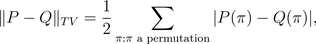
where P(π)
and Q(π)
denote the respective probabilities of seeing the configuration π. It
can be shown that this distance is a number between 0
and 1. It can also be shown that this distance is the largest possible difference between the probabilities that
the two probability distributions can assign to the same event. In the
example above, all the possible 16 configurations of 4 cards after 1
riffle shuffle have the same probability equal to 1/16.
There are 4!=24
possible permutations of 4 cards. Hence the total variation distance
between the distribution after 1 riffle shuffle and the distribution of
a perfectly random deck (for which all permutations have
probability 1/24)
is equal to 1/2*(1/24*8+16*(1/16-1/24))=1/3. The
following table gives the total variation distance for different
numbers of shuffles of decks with different number of cards.
| Cards\Shuffles |
1 |
2 |
3 |
4 |
5 |
6 |
7 |
8 |
| 25 |
1.000 |
1.000 |
0.999 |
0.775 |
0.437 |
0.231 |
0.114 |
0.056 |
| 32 |
1.000 |
1.000 |
1.000 |
0.929 |
0.597 |
0.322 |
0.164 |
0.084 |
| 52 |
1.000 |
1.000 |
1.000 |
1.000 |
0.924 |
0.614 |
0.334 |
0.167 |
Observe that, as Larry explained in the episode, for a regular
deck with 52 cards the deck starts becoming random (i.e. the total
variation distance is less than 1) after 5 shuffles and after 7
shuffles the
total variation distance is less than a half. After this point, the
total variation distance decreases by approximately a factor of 2 after
each shuffle. When the number of cards in the deck increases
towards infinity the graph of the number of shuffle vs. the total
variation distance to the uniform distribution starts looking like the
graph shown in the figure below.
In a subsequent paper titled
"How
many shuffles to randomize
a deck of cards?", L.M. Trefethen and L.N. Trefethen
argued that by measuring the approximation to randomness with
entropy
instead of total variation distance, it takes only approximately
log2n
shuffles to randomize a deck of
n
cards. Hence in this sense only 6 shuffles are enough to randomize a
deck with 52 cards. Diaconis responded explaining that you only need
four shuffles for un-suited games such as
blackjack.

This phenomenon is known as the cutoff
phenomenon. The number K
is known as the cutoff
time. Persi Diaconis and Dave Bayer proved in
1992 in a famous paper titled "Trailing
the dovetail shuffle to its lair" that the cutoff time for
a deck with n
cards is given by (3/2)log2n,
where log2n
denotes the logarithm in base 2 of
n
(see Tangent).
- Activity 2
a) In the top in at random shuffle the top card in
the
deck is removed and
placed back in the deck
at a random position. Persi Diaconis and David Aldous proved in 1986 in
a paper titled "Shuffling cards and
stopping times" that the cutoff time for this shuffle is n
log n, where log n
denotes the natural logarithm of n.
Calculate the total variation distance to perfect randomness after one
top in at random shuffle of a deck with 4 cards.
b) Calculate the total variation distance to perfect randomness after 2
riffle
shuffles of a
deck with 4 cards.