Numb3rs 207: Convergence
It has been stated in Numb3rs that Charlie Epps published his first paper
in the American Mathematics Journal at the age of 14 on the "Asymptotics
of Hermitian Random Matrices" - making him, at least in the Numb3rs universe, the
youngest person to ever publish a major paper! Although perhaps in real life
Carl Friedrich Gauss,
James Maxwell, and
Evariste Galois might have Charlie
beat in child prodigy status, Charlie's main focus in his early research was in
studying a phenomenon which came to be called "the Epps Convergence."
In Episode 207, "Convergence," an old college rival comes to CalSci (Marshall
Penfield, played by Colin Hanks,) to present new research on a gap he has found
in Charlie's proof. Although Charlie does find a way to resolve the error term,
it isn't clear to many people watching still what type of math Charlie really
does do! What he studies falls into the area of probability and statistics
involving what are called "random matrices." While the first activity has no prerequisites,
the latter activities all assume some basic knowledge of linear algebra, matrices, and determinants.
What is a "Random Matrix" Anyway?
Before we talk about what it means to be a "random matrix," let's talk a little
bit about what we're going to mean by "random." If we flip a coin, we "randomly"
choose between two options - heads or tails. If we roll a die, we "randomly" choose
between six options - one, two, three, four, five, or six - each with equal chance
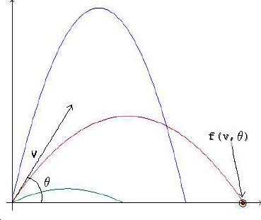
of occurring. However, say we throw a tennis ball in the air ahead of us, at a "random"
angle and with a "random" speed. Where does the tennis ball land "randomly"?
Although linear algebra is a course in its own right, if you
would like to read more a bit more about matrices and vectors in general
before trying out some of the activities, check out either
here
or
here.
The former is a brief refresher article, while the latter is a very basic,
free textbook available online. Similarly, for a more in depth treatment on
basic probability and random variables, check out
here and
here.
Activity 1: Many of you may already know how to work
out where the tennis ball lands given a fixed launch angle and a fixed launch speed,
using the equations
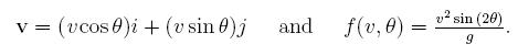
We know that
f(v,theta) is the range, i.e. the place that our tennis ball will
strike the ground if thrown with speed v and at angle theta, so let's see what the "random"
set of possibilities can be. Assume that all speeds are between 10 m/s
and 40 m/s, and assume that we throw somewhere between 0 degrees and 90 degrees
(i.e. straight across or straight up in air.) If all speeds and all angles are equally likely,
calculate:
- All possible values that f(v,theta) can achieve (all possible places that the ball could land!)
(Hint: What's the farthest the ball can go? What's the closest place it can land?)
- If we can only throw at 10m/s, 20m/s, 30m/s, and 40m/s, and only at the angles
(in degrees) 45,60, and 90 (all equally probable) what is the average distance traveled
by the tennis ball? What happens if you have more possible speeds or more possible angles?
- Challenge: Find the average distance that the ball travels, i.e.
the expected value of our "random" f(v,theta) across ALL possible speeds v between 10 and 40 m/s,
and all possible angles between 0 and 90 degrees. Use

noting that p(v,theta) is the probability of us shooting with a fixed (v,theta) out of all
possible options. How does this look like the sum you used for the average in part 2?
You may have noticed something about the first activity - it doesn't really reflect real life.
In real life, if you were going to throw a tennis ball ten times (forgetting the angle for the moment)
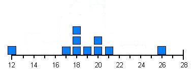
you're probably not going to have every speed between your "top" speed and your "worst" speed be equally likely. It's much more likely that you'll throw, perhaps, with speeds (in m/s) something more like 20,17,18,12,18,26,19,21,20, and 18. Let's see how this looks.
If we graph this, we get something that looks like this:
Say we throw the ball another twenty times. Maybe our distribution of speeds will look something like this:
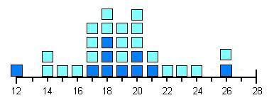
This is more like it. Although sometimes you can throw the ball really fast, and other times your throws will be kind of slow, on the whole, you're likely to throw the ball not too far away from some normal speed for you. Eventually, if we continued this, we'd probably get something that looked more and more like this:
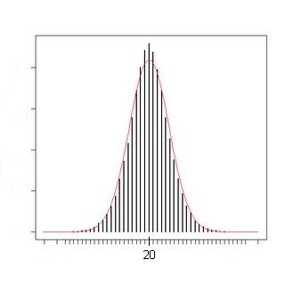
If we normalize, i.e. set the area under the curve to be 1, this is an example (perhaps the most famous example) of what is called a "probability distribution."
What is a Probability Distribution?
Well, we would like a function from our set of possible events - in the case of the previous example of tennis ball throwing, we would mean all possible speed/angle pairs - to real numbers between 0 and 1, so that when we sum this function over
all possible events, we get 1. Essentially, we want this to be true because we'd like to always know that
something happens, i.e. the probability of
something happening is 100%. To read more about the properties of probability distributions in general, look
here.
Specifically, from now on we are going to be mostly concerned with the probability distribution we just saw - the Normal distribution. Here's the most general formula for a Normal distribution:

Those new letters up there, m and s (which are short for "mu" and "sigma," the traditional Greek letters,) help us set where the center of our distribution is - that's exactly m - and set how wide our distribution is. From now on though, we'll be sticking with a distribution with m=0 and s=1, so our Normal distribution will be:

Where else does the Normal distribution show up? Well, lots of places. For example, if you look at a graph of the heights of a representative sampling of humans, that will form a normal distribution. The
Central Limit Theorem tells us that in a huge number of natural and behavioral sciences, the Normal distribution is going to be the most common probability distribution we'll encounter. To get an idea of why real "randomness" is often distributed this way, check out
here and
here.
Now we're ready to talk about what "random matrix" really means. Let X be an NxN matrix with real (or complex) entries, such that each entry is an independent random variable with the "special" normal distribution above. We also require that X be "self-adjoint" (also called "Hermitian",) which means that

The bar over the X^T indicates complex conjugation, so if we are working over the real numbers, this reduces to

Activity 2: What does "Self-Adjoint" or "Hermitian" really mean?
- Which of the following are Hermitian?

- Compute the eigenvalues of the following Hermitian matrices. For the last one, as it involves a quartic equation, you may use this. What do you notice about them? Are they real? Imaginary? Do you think this is always true?

- Using the fact that for Hermitian matrices X=(X^T)* (in this case, * is again complex conjugation,) prove what you conjectured in part 2. Note that if we have a complex number a such that a=a*, we must have that a is real.
- Find an example of a matrix with real eigenvalues that isn't Hermitian.
Wigner's Semi-Circular Law:
Classical probability theory has in a central position the Normal distribution. When we move to
free probability - probability with random variables that do not commute at all - the distribution that fills the same role is Wigner's
semi-circular distribution, given by the following equation:

It looks something like this, although after we normalize, it becomes more of a semi-ellipse than a semi-circle! Note that these random matrices we've been considering
do not commute, so it makes sense that their eigenvalues would be distributed this way instead of in a classical, Normal distribution.

One of the standard results of random matrix theory involves the distribution of eigenvalues of these matrices. At this point, hopefully you've all shown (or at least believe) that all eigenvalues of a Hermitian matrix are real. So, specifically, the eigenvalues of our special NxN Hermitian matrices with independent, normally distributed entries should all have real eigenvalues.
What is the distribution of these eigenvalues as N approaches infinity? Perhaps your first intuition is to guess that they will be normally distributed, in the same way the entries of the matrices are. Unfortunately, that's not even close to true. The eigenvalues will, in the limit, distribute themselves according to something known as "Wigner's Semi-Circular Law." As you may have guessed from the name, that means their distribution - instead of being a bell-curve, like our Normal distribution - is a half circle!
The distribution of these eigenvalues as N approaches infinity is one "asymptotic" that mathematicians study. Another asymptotic, with some very interesting combinatorics behind it, is the distribution of the trace of the nth moments of the matrix as N goes to infinity again.
As a brief reminder, the "trace" of a matrix is the sum of the elements on the diagonal. The kth moment of our matrix X is just its kth power.
Activity 2: Normalizing the Semi-Circular Distribution:
How do we figure out the normalization factor for the semi-circular distribution? Let's work it through.
- First, what is the equation for a semi-circle whose center passes through (0,0) with a radius of R? In polar coordinates? In Cartesian coordinates? For Cartesian coordinates, just write the equation for y>0 or y=0. You should have a function f(x) defined between -RNext, integrate your equation between -R and R. What value do you get? Call this N.
- Can you figure out the integral of your semi-circular equation without actually doing any integrating?
- Note that if you take f(x) and divide by N, you will have a new function defined between -R and R, this time with integral 1 when evaluated between -R and R. Check that this matches up with Wigner's semi-circular distribution above!
Asymptotics of Random Matrices
This other asymptotic of interest, the "expected" (i.e. average) value of the trace of the kth order moments of our NxN matrix as N goes to infinity, can be written as follows:

where X^N means that X is an NxN matrix, while we are taking the trace of the kth power of X. We can expand out the various powers of this, an integrate across our N^2 degrees of freedom, and an amazing result comes out - the only terms that remain after expanding out are counted by non-crossing pairings of k things sitting in a circle. Hence, if k is odd, we can show that in the limit this must be zero (as there are no possible pairings of k things if k is odd.) If k is even, the number of non-crossing pairings is counted by the Catalan numbers! The Catalan numbers are defined by

and count an amazing array of things - rooted binary branching trees, triangulations of polygons, non-crossing pairings of 2n things, non-crossing partitions of n things, Dyck paths, and many, many other seemingly different groups of objects.
Binomial Coefficients:
Recall that the notation

is read as "n choose k", and it counts the number of ways that you can pick k things out of n things, regardless of the order of your choice. It can be computed by:

To read more about this, refer to
here or
here.
While the proof that the following equation holds can be found here by showing a connection to rooted binary branching trees, perhaps the easiest combinatorial proof is in [1], where a bijection with non-crossing pairings of n things is proved very neatly:

Essentially, the proof amounts to expanding out the trace in terms of the X_{i,j} and showing that all of the terms in this sum can be indexed by partitions of k things. Then, we show that all of the terms which do not correspond to pairings have to integrate to zero - and finally, all of the pairings which have crossing elements also integrate to zero.
Each of the terms we have remaining then correspond to a non-crossing pairing, and we can then show that each of these integrals is 1 - hence, we have a contribution of 1 to our total sum for each non-crossing pairing, and there are C_k of them!
Activity 4: What are the Catalan Numbers?
- First, prove the following equality either by manipulating the binomial coefficients or by making a good combinatorial argument:

- We have the definition of the Catalan numbers up there. However, there are a number of ways of defining them. Show that we can also write them as

again, either by manipulating the binomial coefficients or by making a combinatorial argument.
- Challenge: The Catalan numbers can also be defined by the following recurrence relation:

Using this, show that the number of non-crossing pairings (see below) of 2n things is the nth Catalan number.
Non-Crossing Pairings
If we place
2n things on a line (or place them around a circle) we say a non-crossing pairing is a way of matching up every element on the line with some other element so that every element is paired and no lines which pair two different pairs of elements cross. By way of example, for four elements, there are only three pairings.
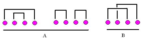
The two on the left, labeled "A", are non-crossing. The one on the right, labeled "B", is a crossing pairing. So there are only two crossing pairings of four things.
Can you draw the number of non-crossing pairings for six things? How about for eight? Notice that if you start to draw a pairing, and you try to connect the first element to an element that is an even number of steps away, you
can't finish your pairing! Why?
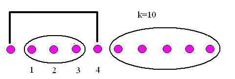
Here are a few completed matchings for
k=10, drawn on a line and on a circle (the asterisk denotes the first element in the corresponding non-crossing pairing drawn on the line.) Can you see a way of breaking up each of these into smaller non-crossing pairings? Can you use this to prove part 3 of activity 4?


References and Further Reading:
[1] Speicher, R. Lectures on the Combinatorics of Free Probability
[2] Guionnet, A. Lectures on Random Matrices: Macroscopic asymptotics
[3] Stanley, R. Enumerative Combinatorics I - An excellent reference if you'd like to see up to 66 places the Catalan numbers appear.