In the interview at the very beginning of the episode Charlie mentions that he may be able to extract an egress path based on traffic flow data. Here we will discuss one method to accomplish this, using Markov Process modeling.

(It may be useful to first read the math behind Episode 113)
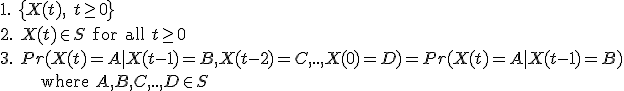
A Markov Process is a model used to represent memoryless processes in time. These processes can be either time homogenous (Discrete Time Markov Process) or non-homogeneous (Continuous Time Markov Process). Due to the higher complexity of the latter case, here we only concern ourselves with the discrete case.
Now we define the Discrete Markov Process formally (from here Markov Chain will mean Discrete Time Markov Chain):
Translation: (1) and (2) form the basic definition of a state time process (another important subset is a State Machine), where for any time t the process X(t) can be in one of the states defined in the state space S; (3) defines the memoryless property (note that A, B, C, D are not necessarily different states). Transitions between states occur at discrete time steps (hence the name).
Another subtle point here is that the third line implies that the sum of probabilities of entering any state given the previous state must sum up to 1 due to the definition of probability.
The typical method of defining a Markov Chain is to define its time domain (identically to (1) above), its state space, and a probability matrix. For example:

The rows of D denote the current state and the columns the probability of entering the corresponding state at the next time change. For example  .
.
Note that once the process enters state 3 it can never leave: state 3 may be referred to as an absorbing state. One can also view this simple process as a directed graph to gain intuition:

The dashed edges (also called loops) are optional because their values are implied by the fact that the values of the outgoing edges must sum up to 1.
A useful analysis at this point is classification. We can sort the states into one or more disjoint and non-empty subsets of states that communicate with each other. In this case, there are two classes: {1,2},{3}. It easy to see from the diagram that there is a path from 1 to 2 and from 2 to 1, therefore they communicate. However, even though there are paths from 1 and 2 to 3, there is no return path, therefore they do not communicate: the only state that communicates with 3 is itself.
Consider a Markov Chain with the following state space and probability matrix:

In any modeling problem, we simplify the real world into mathematical entities. If we were to compute a probable egress path using a Markov Chain, we need to only assign locations to states and then use traffic flow information to assign transition probabilities to other states. For example, take the chain defined in the activity above. The states could correspond to an office building (1), a mall (2), a pair of hospitals (3,4), an entry into town (5), and neighborhoods (6,7). This would suggest that once you get sick, you just get bounced between hospitals for ever, the first neighborhood is larger (more people go back there) and no one leaves once they come to town. Of course, this situation is absurd, but it does illustrate the possibilities of this modeling technique.
As you may have already guessed, the transition probabilities are used in a matrix form for a good reason. Lets suppose we want to see what happens to a new-comer once she enters town (X(0) = 5). We simply define a row vector v = (0 0 0 0 1 0 0) and multiply it by D. vD = (1 0 0 0 0 0 0). The resulting vector gives the probabilities: 
For the probabilities

we need to simply compute vDD to get (.1, .2, 0, 0, 0, .6, .1). For the next time step, t = 3, we compute vDDD = (.14, .12, .02, .02, 0, .6, .1) and so forth.
The above does not violate the memoryless property. Can you explain why?
Note that this method of computation is only useful if we have a finite state space. Can you explain why? For an example of an infinite state space look at the "evil but useless robot" example in Episode 113
A more realistic model will likely have numerous locations such as street blocks, intersections, and highways. The transition probabilities will be based on the traffic flow data. Then the initial position of the "suspect" would be modeled the same as above, and then a time-driven probability distribution can easily be computed from that. The difficult part comes in actually interpreting the resulting information: would the person return to the initial position? would she take the road less traveled or try to get lost in the crowd?
This last interpretive step is necessary in all modeling scenarios as all models are almost always wrong but sometimes useful.
* For further reading on probability models, texts by Sheldon M. Ross (there are many, and most all are useful) are commonly referred to by most beginning and intermediate students.