
Sudoku and logistic regression. They have two things in common: both appeared in this episode of Numb3rs, and both involve some interesting math. What math? Great question! Read on and find out.
Although Sudoku first became popular in Japan, it was in fact invented
by an American, Howard Garns, in 1979. The goal is to place the numbers
1 through 9 in square cells of a 9x9 board such that
.png)
One of the first seriously study the mathematics of Latin squares was the prolific 18th century mathematician Leonhard Euler (OIL-ler), who was intrigued by the following puzzle: given six different regiments that each have six officers, each of one of six different ranks, can these 36 officers be arranged in a 6x6 square so that each row and column has one officer of each rank and regiment? To make this clear, let's mark each regiment by a different color, and denote each of the six ranks by the corresponding die side (see picture below). The question then becomes, can one arrange the dice on a 6x6 board such that each row and column has a die of each color and face value?
.png)
.png)
In trying to solve the original 6x6 officers puzzle, Euler noticed
that the resulting square would break up into two Latin squares, a
square of colors and a square of dice in our example. .png)
Thus all one needs to do to solve the six regiments problem is find a
pair of Latin squares which when put together satisfy Euler's
requirements, i.e. when the squares are superimposed, each pair of
symbols (or die values and colors) occurs exactly once in the whole
square. Such pairs are called
Graeco-Latin squares, for the simple reason that Euler denoted the
elements of one by Latin letters and the other by
Greek. After some tinkering, Euler wasn't able to find a 6x6
Graeco-Latin pair, and he conjectured that such pairs don't exist for
any n=4k+2, where k is an integer bigger than 0.
It wasn't until 1901 that a mathematician showed, by exhaustive
enumeration of 6x6 Latin squares, that a 6x6 Graeco-Latin pair
truly doesn't exist. Euler's overall conjecture, however, was shown to
be false in 1959: Graeco-Latin pairs exist for all n except 2 and
6.
Consider the pair of Latin squares below. Are they Graeco-Latin? We make a single 4x4 square by adding the corresponding entries of the pair. The result is called a magic square. It's a square with distinct integer entries such that the sum of each row, column, and diagonal is the same, in this case 34.
.png)
 Perhaps the most famous magic square is the one reproduced
below. This 4x4 square
appears in Albercht Dürer's 1514 engraving Melencolia
I, to the right. What other mathematical objects
can you find in Dürer's engraving? What do you think is
the idea Dürer tried to convey?
Perhaps the most famous magic square is the one reproduced
below. This 4x4 square
appears in Albercht Dürer's 1514 engraving Melencolia
I, to the right. What other mathematical objects
can you find in Dürer's engraving? What do you think is
the idea Dürer tried to convey?.png)
As you may already know, The
Acme Corporation's yearly production of anvils depends
heavily on the amount of iron Acme mines. Here's a data table
summarizing the last decade: .png)
Unfortunately, Acme's mining business is in some trouble this year, and
is expected to produce only 460 tonnes of iron. Naturally, Acme's CEO
wants to know how many anvils can the factory expect to produce, and
you've been given the assignment of figuring this out.
The first thing you decide to do is graph the points, like this. .png)
After some thought you come up with the following bright idea: all
that's needed is a curve, based somehow on the existing data, that will
show the correspondence between iron mined and anvils produced.
.png)
.png)
After trying the above naive approach, you consult a book on statistics and find the method of linear regression. The essence of this method is to fit a line to the existing data points so as to minimize the squares of the vertical distances between the line and the points (see illustration to the right). Why the squares of distances and not simply the distances? Mostly out of mathematical convenience irrelevant to this discussion, details which you'll likely cover in an intermediate level statistics class.
An equation of a line in the plane has the form

for some y-intercept a and slope b. What we would like to do is find a
way to write the slope b and intercept a of our regression line
in terms of the given data points (xi,yi) (in our
case indexed by i=1997, 1998,...,2006). In fact, using
a bit of calculus it can be shown that 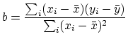
and

where  is the average of the xi and
 is the
average of yi. Keep in mind that while you can always fit a
regression line to a set of data, the line might not tell you much if
the points of your data are not "close" to being on a single line but
are scattered all over; it will have no predictive power. On the other
hand, in our case of anvils and iron, there's a pretty good linear fit.
There's an exact way to quantify how well a regression line fits the
data, but that's a story for another day (or wikipedia).
is the
average of yi. Keep in mind that while you can always fit a
regression line to a set of data, the line might not tell you much if
the points of your data are not "close" to being on a single line but
are scattered all over; it will have no predictive power. On the other
hand, in our case of anvils and iron, there's a pretty good linear fit.
There's an exact way to quantify how well a regression line fits the
data, but that's a story for another day (or wikipedia).
In this episode, Charlie proposes to find how likely someone is to commit a terrorist act based on various variables (money, fanaticism, etc.) using logistic regression. In general, logistic, as opposed to linear, regression is used when you're dealing with a binary--yes/no, pass/fail, 0/1, etc.--dependent variable (the variable you're trying to predict based available data). Here's an example that will make this clear.
.png)
Suppose you would like to know how likely a young law school graduate is to pass the bar exam based on how much time they spent studying for it. Further suppose you have the relevant data from last year's 27 exam takers, graphed on the right with pass and fail on the y-axis, and the hours spent studying on the x-axis.
.png)
.png)
In the 1970's statisticians were mulling over
question #2 above, and what they came up with is logistic
regression. The idea is to approximate the data by an "S" shaped
curve, called logistic curve, that looks something like the curve on the
right, and is given by the following equation,
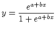
where e is the base of the natural logarithm, and a and b are again
parameters, but this time not as simple to interpret as intercept and
slope in case of linear regression.
A good way to think about logistic regression, and a very good way to actually approximate it, is as linear regression in disguise, the disguise being the natural log function.
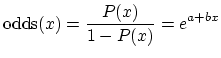
The odds of an event A, say flipping a coin and getting tails, is the
probability of it happening divided by the probability of it not
happening,
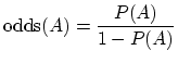
Thus if we know the odds of an exam taker passing after studying 120
hours, we can calculate the probability of passing through simple
algebra. So without any loss of information, we shift to working with
the odds instead of the probability, thinking of odds as a function of
events, just like we treated P.
.png)
As you've seen in part #3 above, the log odds look much more like the continuous dependent variable we used linear regression on earlier in this section. So that's just what we'll do now: use linear regression on the log odds! From our data we can divide the range of hours studied into suitable intervals (of say 40 hours), and count the odds for each interval as (#points at 1)/(#points at 0), as on the right. We then graph the log odds, treating each of the 5 different values we got for the intervals as multiple points according to how many original data points fell into the corresponding interval.
.png)
Finally, what we get is a regression for the log odds of the form
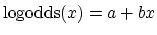
as before when we did linear regression. Taking the base of the natural
logarithm e to the power of both sides, we get
and solving for P, we get the equation of the logistic curve!
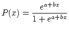
Thus the
orange regression line to the right is mapped by the transformations
above to the logistic curve approximating our original data.
The actual calculation of the logistic curve coefficients is done differently, usually by calculators or computers, but this procedure is simple, conceptually enlightening, and very close to the actual best-fitting logistic curve.