Auction Theory 

In this lesson we will state the first important theorem of auction theory, commonly known as the Revenue Equivalence Theorem. Before doing so, we will generalize some results obtained in the previous lessons to the case when valuations are continuous random quantities with certain properties. In order to do this it is important to recall the concepts of distribution and density functions for a continuous random variable.

Distribution and density function

Given a continuous random variable X, the distribution function of X, denoted by F, is defined by the formula



When this function is differentiable, we say that X has a density function which is defined by the formula



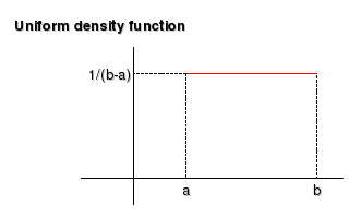
For instance, if X is uniformly distributed on [a,b] the density function of x is f(x)=1/(b-a) if a≤x≤b and f(x)=0, otherwise (see figure).

Expected revenue in the English and Vickrey's auctions

We observed in lesson 2 that under assumptions A1-A4 the revenue of the seller in the English and second-price sealed-bid auctions was equal to the second highest valuation among bidders. In terms of the order statistics this revenue is equal to v_(N-1), where N is the number of bidders. Assuming that the valuations have a density function, f, with some nice properties, it can be proved that



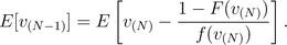
In fact, we already have used this fact in lesson 2 for the specific case of the uniform distribution.

Expected revenue in the Dutch and first-price sealed-bid auctions

In lesson 3 we observed that assuming a Dutch or first-price sealed-bid auction has two bidders whose valuations are uniformly distributed on [0,1]. Under hypotheses A1-A4, the Bayesian Nash equilibrium for each bidder is to bid half of his/her valuation. This result can be generalized to the case of N bidders whose valuations have a common density f, with some nice properties. It can be proved in this case that a Bayesian Nash equilibrium for player i is to bid



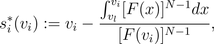
where v_l is the lowest valuation each bidder can have (if the bidder bids less than this quantity he/she has zero surplus).


Hence in terms of the order statistics the expected revenue of the seller in this case is equal to



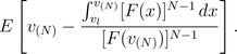
It can be shown that this quantity is equal to the revenue of the seller in the English and Vickrey's auctions (formula above), which leads to the following theorem.

The Revenue Equivalence Theorem

For the benchmark model, with hypotheses A1-A4, each of the English auction, the Dutch auction, the first-price sealed-bid auction, and the second-price sealed-bid auction yields the same price on average.


There exists however a fundamental difference bewteen the equilibrium in the English and Vickrey's auctions and the equilibrium in the Dutch and first-price sealed-bid auctions. In the latter, the equilibria are dominant equilibria in the sense that each bidder has a well defined bidding strategy regardless of how high his rivals bid. In the former, the equilibrium for each bidder is optimal given that his/her rivals are using the same decision rule (Bayesian Nash equilibria). Also, recall that in the English auction the seller never discovers the winner's valuation, but in the second-price sealed-bid auction the winning bid is actually equal to the highest valuation. Hence, although the average revenue in all the auctions is the same, there exist properties that are different for the different types of auctions. Also, if some of the assumptions A1-A4 are dropped the outcome of the auctions could change substantially. For instance, when assumption A2 is dropped we have the following result.

The winner's curse

Suppose A1, A3, A4 hold but instead of having hypothesis A2 (independent-private-values assumption), there is a common value of the item that is unknown for all bidders. In this case, for a sealed-bid auction each bidder makes an estimate about the true value of the item. The bidder with the highest estimate will win the auction (why?). But this means that the winner of the auction overestimated the value of the item, since everybody considered it to be less, and hence he/she might end up overpaying. A more formal statement of this result uses conditional probabilities and it is out of the scope of these lessons. Hence by dropping A2, the winner of the auction might lose the rent he/she would win if A2 were satisfied.

A double auction

Double auctions are used for example in the stock market as described in lesson 1. Here we present a very simple version of a double auction where there is one seller and one buyer who have private information about the value of item. The seller names an asking price p_s and the buyer an offer price, p_b, simultaneously. A transaction occurs if and only if p_b>p_s, and in this case the price paid for the item is equal to p=(p_s+p_b)/2. Assuming that the valuations of seller and buyer, are uniformly distributed on [0,1], a Bayesian equilibrium for this auction is given by the formulas



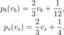
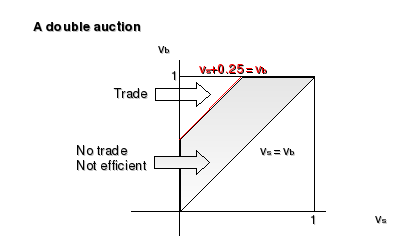
As a consequence, in this equilibrium trade occurs if and only if v_b≥v_s+(1/4) (see figure). It can be shown that there is no Bayesian Nash equilibrium that is efficient in the sense that trade occurs if and only if v_b≥v_s. This auction is different than the ones presented in the previous lessons in that the seller also takes part in the auction by submitting an asking price.

Further reading

The results presented in these lessons are merely introductory. Further results are obtained by relaxing hypotheses A1-A4. Also auctions are a particular example of games with incomplete information, additional results are obtained for sequential games of incomplete information when for instance, bargaining is possible. In this regard, we refer the interested reader to the literature below.

References

1. Gibbons, R. Game theory for applied economists, Princeton University Press, 1992.
2. McAfee, P. and McMillan, J. Auctions and bidding, Journal of Economic Literature 25:699-738, 1987.