The kind of
process we described in the previous section is an example of a very
general kind of processes called
Markov
chains. To describe such a Markov chain, we need the
following data:
First, we have a set of
states,
S = {
s1,
s2,
... ,
sr
}. The process
starts in one of these states and moves successively from one state to
another, in the very same way our mouse moves from room to room in the
maze. Each move is called a
step.
If the chain is currently in the state
si,
then it moves
to the state
sj
at the next step with a probability denoted by
pji
, and this
probability does not depend upon which states the chain was in before
the current state. The probabilities
pji
are called,
once again,
transition
probabilities. While we did not allow it in our first
example, in general, the process can remain in the state it is in, and
this occurs with probability
pii.
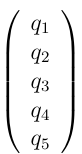
An initial
probability
distribution, defined on S, specifies the starting state.
Usually this is done by specifying a particular state as the starting
state. More generally, this is given by the distribution of
probabilities of starting in each of the states. For example, in the
5-state process describing our mouse, the distribution
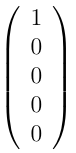
would
mean that the mouse is in the first room at the
beginning of the experiment, while the state
would
represent the starting state of the mouse in the unfair
5-sided die experiment.
We can represent the process with a
graph whose
vertices (nodes)
represent the different states the system can be in, while the arrows
represent the possible steps. Over each arrow we write the transition
probability associated with that step.
Question
Going back to the mouse example, the figure below is part of the
graph representing the mouse process. Can you complete it?

Such a graph makes it easy to visualize the process, but what really
makes Markov chains a computationally efficient framework is the matrix
representation.
We write the transition probabilities in an array as follows:

This means that to find the transition probability from state
i to state
j, we look up the
initial state on the
top
line and the new state on the
left. The number at
the intersection of that row and that column and the transition
probability we’re looking for.
Question
Write the transition matrix for Little Ricky in the maze.
The power of this framework comes to light when one realizes that
equations (3) and (1) are nothing but a rewriting of the
multiplication rule for vectors
and matrices. In summary if we rewrite what we showed in
the previous section using this matrix language, we can prove the
following theorem:
Theorem:
Fundamental Theorem of Markov Chains
If P = (
pij)
is the transition matrix for a Markov chain and
q =
(q1...qn)
t
is a distribution
of probabilities on the states of that chain then:
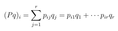
- (i) The distribution of probability values on
the states after 1 step
starting on s
is given by the matrix-vector product P q where the ith
component of
the new vector is given by:
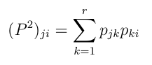
- (ii) The probability of ending up in state j after 2 steps
starting from state i
is given by (P2)ji
where
P2
denotes the product of the matrix P with itself. Explicetely:
- (ii’) More generally, the transition
probabilities after n
steps are given
by the transition matrix Pn,
the n-fold product of the matrix P
with itself.


