The Laplacian in Rn is an important operator in differential equations such as the heat and wave equations. In R, the Laplacian is just the usual second derivative. Laplace's equation sets the Laplacian of a function equal to zero. Solutions of Laplace's equations are called harmonic functions. There is a theory of Laplacians and harmonic functions on fractals including the Sierpinski Gasket.
Let u be a function defined on the SG. Then the pointwise Laplacian is defined:
where the sum runs over the four neighbors of x.
The main computational tool is the harmonic extension algorithm which allows us to compute the values of harmonic functions at points within a cell if the cell's boundary values are known. Take the following cell:
If u is harmonic on the cell then
and similarly for u(q12) and u(q12).
Another known formula used is:
The family of functions I studied have a singularity at a periodic point so they are harmonic everywhere except at a point. The family has 6 members since the space of harmonic function with the a singularity at this periodic point is 6-dimensional. In order to create a singular function on the SG we must have a self-similar contraction around the singular point. Also, the value of the harmonic function at an interior point must be the average of its neighbors. The third condition imposed was a matching condition for the normal derivatives. Normal derivatives on the non-boundary points are defined by the pointwise equation:
where the sum runs through two (of the 4) neighbors of x which are in the same cell of level m. Thus there are two normal derivatives at such a point (in opposite direction) and they must be equal in magnitude and opposite in sign.
Using the two equations above for finding the values of harmonic functions I solved equations for the values at all the points of level 2. The only trick was computing the 6 point values labeled in the following figure to determine the unique function.
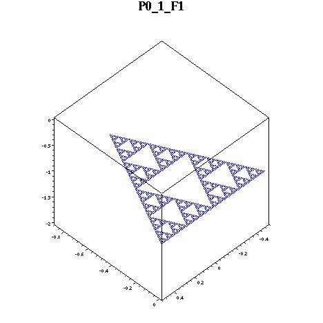
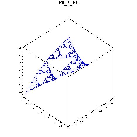
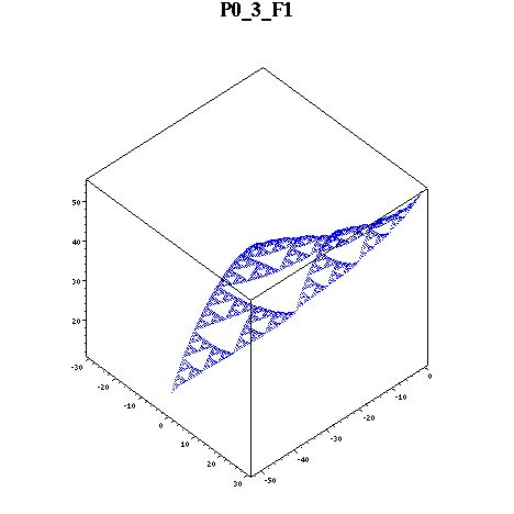
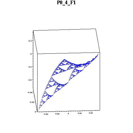
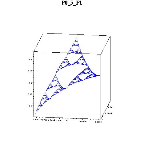
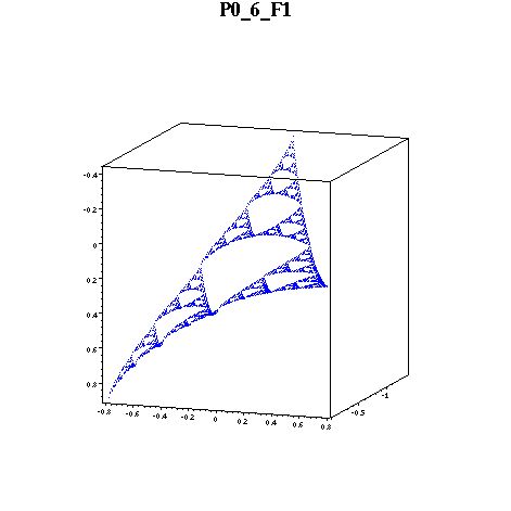
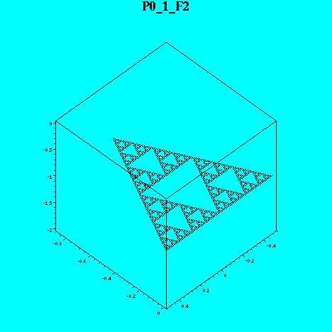
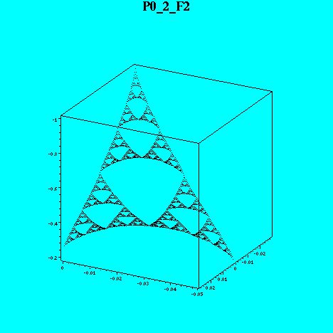
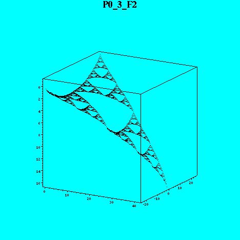
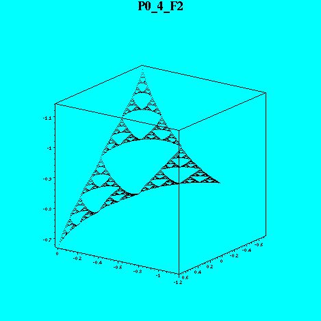
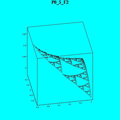
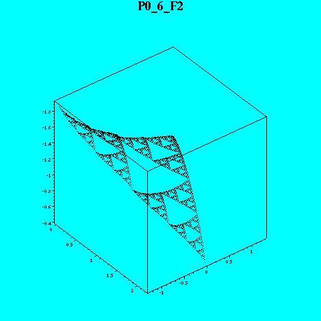
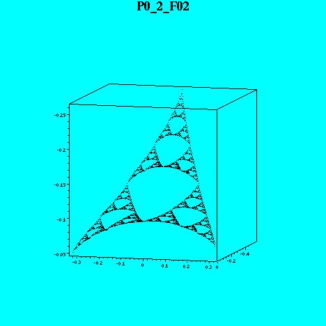
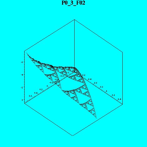
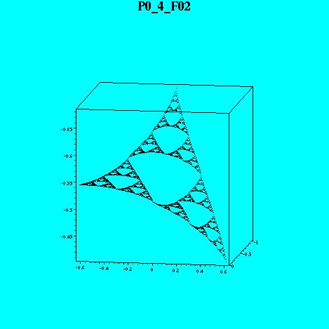
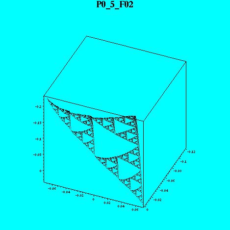
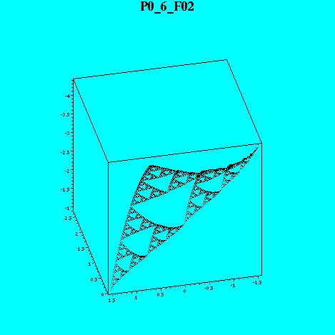
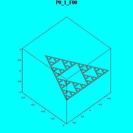
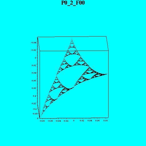
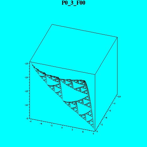
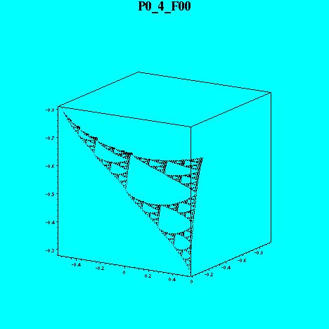
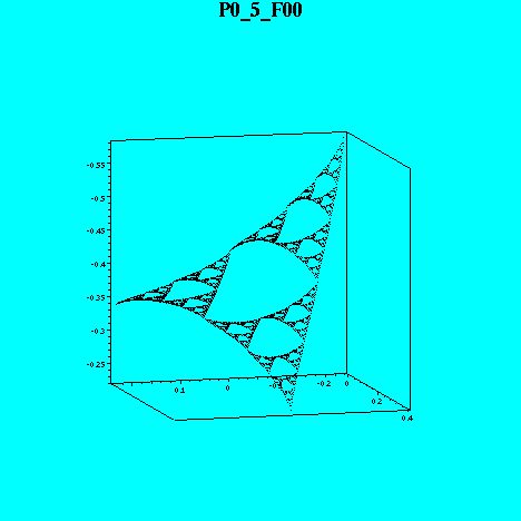
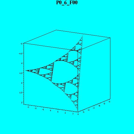
The 6 functions are very distinct. The first three, called P01 through P01, actually do not have a singularity but they have self-similarity about the periodic point. P01 is the constant function. P02 and P03 have removable singularities. The second three have genuine singularities. P04 has a vanishing singularity and relates to the Green's function. P05 and P06 have pole singularities. These qualities of the 6 families
My Maple code that computes the 6 different basis functions up to level 2 is located here. I used the equations:
pts1 := (c0,c1,b2,a0,a2,a1): b1 := (25/56,5/56,3/56,5/56,15/56,3/56).pts1: c2 := (81/224,61/224,3/224,61/224,15/224,3/224).pts1: b0 := (25/224,5/224,59/224,5/224,71/224,59/224).pts1: d0 := (45/224,9/224,83/1120,9/224,639/1120,83/1120).pts1: d1 := (15/112,3/112,13/112,3/112,65/112,13/112).pts1: d2 := (25/112,5/112,71/560,5/112,243/560,71/560).pts1: e0 := (5/224,1/224,507/1120,1/224,71/1120,507/1120).pts1: e1 := (5/112,1/112,283/560,1/112,71/560,171/560).pts1: e2 := (5/112,1/112,171/560,1/112,71/560,283/560).pts1:
Vertex names are labeled in this picture. A rather simple way to display these functions is to execute this worksheet. The datatyping could definitely stand some improvement.
More accurate graphs of the cells are below.