Multiharmonic Functions

Multiharmonic functions are those that are killed by higher iterates of the Laplacian. I computed multiharmonic functions on four cells which did not include the the singularity by taking linear combinations of the three families of continuous harmonics computed by Jonathan Needleman. This required solving for four families of coeficients a_l,n,k , b_l,n,k , c_l,n,k , d_l,n,k using this Maple file.

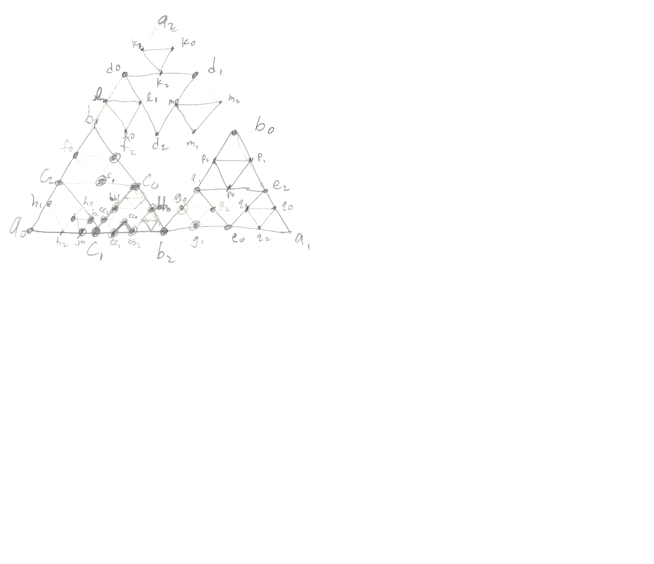
I solved for the l=0 coefficients separately using these matrix equations. Essentially, its 4 3 by 3 systems written sloppily coefs=invC.v . When coefs=(a01k,a02k,a03k), v=(b2,a1,b0). When coefs uses the b's in the same order, v=(a2,b1,b0). When coefs uses the c's in the same order, v=(c2,c0,b1). When coefs uses the d's in the same order, v=(a0,c1,c2). Again, variables names used in the v vectors above are labeled in this picture.

For each j>0 and k I had to solve the following matrix equation Lx=r for x merely by inverting L. See the matrices here .

The ratios of one multiharmonic at a point to the previous multiharmonic there are given here. The rows are different k. The columns are the different points of the cells in the order left, right, top boundary point.

The suspected graph eigenvalues can be computed here.

Then using Needleman's code as a base I produced the multiharmonics in the different cells along with graphs. To produce more graphs use this file.

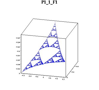
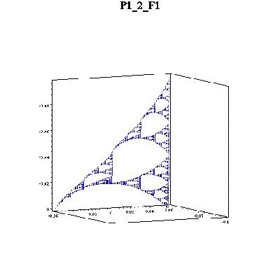
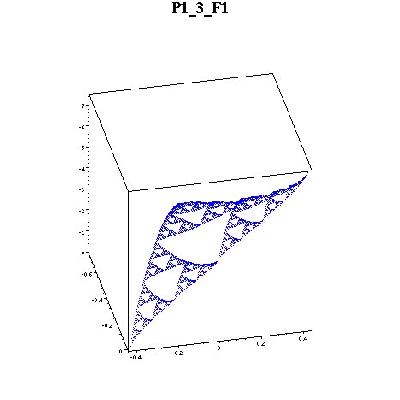
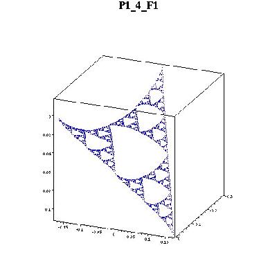
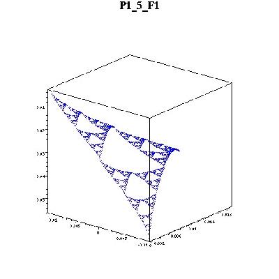
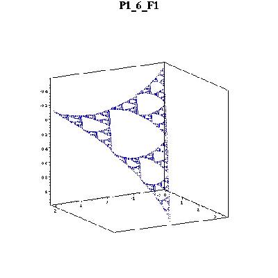
Here are pictures of the 6 biharmonics on F₁(SG). Please ignore the axes values. They are wrong but the graphs are correct. The z-axes values are displayed negative. Anyway, notice that, in this cell, the boundary point on the left (F₁(q₀)) is the closest to the periodic point I studied. The values at that point is near zero. Higher multiharmonic functions will have values at this point (and others) converging to zero.

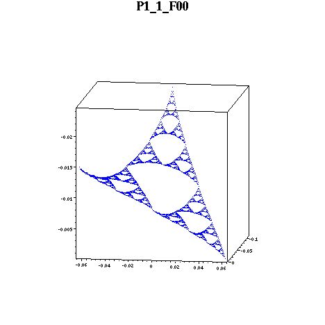
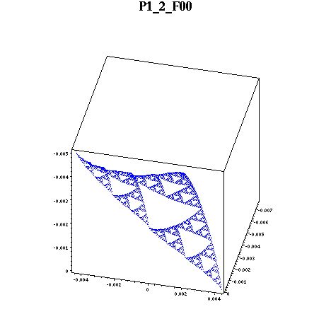
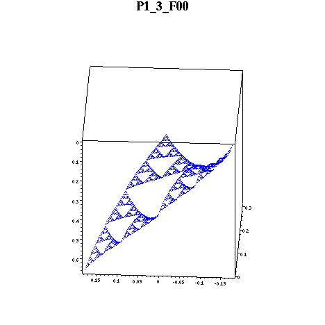
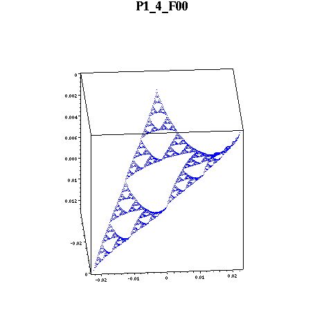
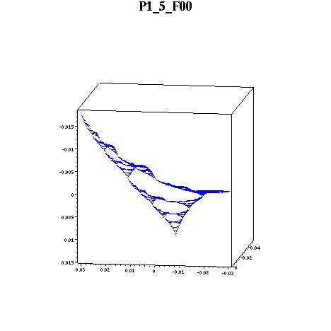
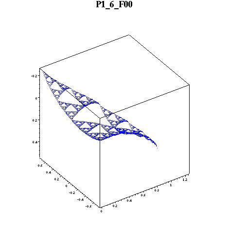
Here are the biharmonics on F₀₀(SG). Notice that the rightmost point is near zero.