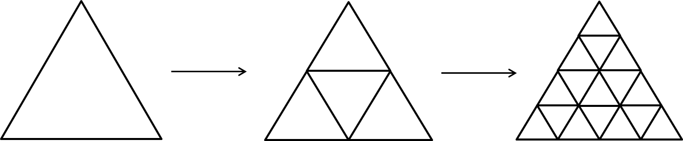
We start with points in an equilateral triangle T. A level 0 partition contains only one cell that contains all the points. A level 1 partition contains 4 cells, each contians points that forms the shape of a smaller equilateral triangles as shown below. We obtain level n+1 partition by splitting each cell of level n into 4 smaller cells in the above fashion.
Given a level n partition of T = \bigsqcup_{i = 1}^{4^n} C_i, we define a random potential P: T \to \{0,P_{max}\} that is constnt on each cell C_i. This random potential is a Bernoulli random variable with parameter p. In other words, each cell independently have a probability p of being assigned a potential P_{max} and 1-p of being assigned no potential. We define the random potential on triangle this way so that it is compatible with that on the Sierpinksi Gasket for convenience of comparison.
Physically speaking, P_{max} simulates the potential caused by structual anomaly in the solid, which happen with probability p. We want to see how does this structural anomaly affect the electron distribution, which is given by the stationary Schrödinger equation as the eigenfunctions of the random Hamiltonian.

We obtain the solutions to the eigen problem Hv = \lambda v as well as the problem Hu = 1 via matlab's pde solver.