Numb3rs 305: Traffic
The main mathematical topic in this episode is the question of determining
whether something is random or not. There is also a brief discussion of
choosing road widths to optimize traffic flow, which is mentioned in a
Tangent.
Randomness
One of the main mathematical issues in this show was determining whether
some particular data set was actually random. Of course, this is impossible
to do with absolute certainty. For example, if someone told you they had
rolled a dice 100 times and gotten a 1 every time, it would be reasonable to
say that either they were lying or the dice rolled wasn't random.
However, it is possible to roll a 1
100 times in a row, so one can't be completely sure that the person
was lying or that the
dice isn't fair. What we would like is a mathematical procedure that takes
some data as input and then outputs a number that indicates how likely it
is that the data is random. For example, given n dice rolls one
could take the sum of all the rolls. Then if n is large, say over 50,
in almost all cases the sum of the dice rolls would be close to
7n/2.
However, in the example above, the sum is 100, which is far from 350. This
would indicate that the data is unlikely to be random. (The pedantic reader
might complain that the proper singular/plural forms are die/dice,
respectively. The choice of the plural form in all uses was made due to the
multiple definitions of the word "die". Hopefully this will not
be too distracting.)
Activity 1:
This is a partner activity. Both you and your partner should follow the
following instructions seperately.
- Write down a series of 20 dice rolls, trying to make them seem
random.
- Find a dice and roll it 20 times, recording the results on a seperate
piece of paper.
- Give both pieces of paper to your partner (and take their pieces of
paper). Try to guess which sequence is random and which was created by your
partner.
Let's study what we just did a little more carefully. First, let's look
at one roll of the dice. This is an example of a random variable. For
our purposes, we will define a random variable as set of pairs (number,
probability) such that the sum of all the probabilities is 1. The first number
in each pair is supposed to be the outcome of some random event, and the
second number is the probability of that outcome. For example,
we could describe the random variable corresponding to a fair dice as
X = {(1,1/6), (2,1/6), (3,1/6), (4,1/6), (5,1/6), (6,1/6)}. The random variable
corresponding to the unfair dice that was rolled in the first paragraph
seems likely to be X = {(1,1)}, i.e. the only possibility is to roll a 1.
In the above paragraph we said that the sum of the rolls we were testing was
100, which was far from the expected value of 350. Now can we describe
this in a more rigorous way? Yes, using the mathematical idea of
expected value (this is one of the cases where the name for a
mathematical concept means almost exactly what it does in normal English).
First we define the expected value, or expectation, of one random variable X.
The formula is 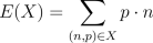 The equation has a couple funny symbols in it, but in words this means
that you take each possible outcome, multiply it by the
probability that it occurs, and then sum all of these numbers up. For a fair
dice with 6 sides, this leads to E(X) = 1/6 + 2/6 + 3/6 + 4/6 + 5/6 + 6/6
= 3.5. Taking the expectetation of a random variable is essentially
figuring out what its average value is.
The equation has a couple funny symbols in it, but in words this means
that you take each possible outcome, multiply it by the
probability that it occurs, and then sum all of these numbers up. For a fair
dice with 6 sides, this leads to E(X) = 1/6 + 2/6 + 3/6 + 4/6 + 5/6 + 6/6
= 3.5. Taking the expectetation of a random variable is essentially
figuring out what its average value is.
Now that we've defined expectation, how can we apply it to multiple dice
rolls, or random variables in general? We'd like to figure out the expected
value of the sum of several dice rolls. To do this, we'll define addition of
random variables in general, and then see how addition interacts with
expectation.
In the episode Larry mentions the quote "Mathematicians are machines for
turning coffee into theorems," which he attributes to Renyi, but has
also been attributed to Erdos, a famously eccentric Hungarian mathematician.
He said it because mathematicians take coffee as input and then are
supposed to output theorems.
Activity 2:
- If expectation is supposed to correspond to averages, what do you
think the expectated sum of rolling two fair dice is?
- What do you think the most common value of the sum of two fair dice is?
- Do Activity 2 in Running
Man. How
do your answers there compare with the answers to the two previous questions?
- Do you have a guess as to how expectation and summation of random variables
will interact?
Now let's define the sum of two random variables X,Y. First we'll give the
formula and then explain what it means in words.  This formula probably contains some symbols you aren't familiar with, so we'll
explain them. First, the outer squiggly braces mean that we are creating set.
In general, the expression
This formula probably contains some symbols you aren't familiar with, so we'll
explain them. First, the outer squiggly braces mean that we are creating set.
In general, the expression 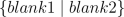 refers to a set. The
elements of the set are described in blank 1, and these elements are subject
to the restrictions listed in blank 2. In this case, the elements are pairs
(m+n,pq), and the restrictions are that (m,p) must be an possible event for
the random variable X and (n,q) must be a possible event for the random
variable Y. An observant reader will notice that we are making an
assumption here that hasn't been stated yet. We are implicitely assuming
that the probability of the event "m and n both happen" is the
product pq. However, this is only the case if the random variables X, Y are
completely unrelated to each other, or independent. For example,
if X is 1 roll of a dice, and Y is a second roll of a dice, then X and Y are
independent, but if X is the sum of a red and a blue dice and Y is the
value of the red one, then X and Y aren't independent. From now on we'll
assume that all of our random variables are independent.
Let's look at an example where X, Y are both random variables
corresponding to a flip of a fair coin with sides labelled by 1 and 2. Since
the possible outcomes of the new random variable X + Y correspond to pairs
of outcomes, one each from X and Y, we can write down the possible outcomes
for X + Y in a table.
refers to a set. The
elements of the set are described in blank 1, and these elements are subject
to the restrictions listed in blank 2. In this case, the elements are pairs
(m+n,pq), and the restrictions are that (m,p) must be an possible event for
the random variable X and (n,q) must be a possible event for the random
variable Y. An observant reader will notice that we are making an
assumption here that hasn't been stated yet. We are implicitely assuming
that the probability of the event "m and n both happen" is the
product pq. However, this is only the case if the random variables X, Y are
completely unrelated to each other, or independent. For example,
if X is 1 roll of a dice, and Y is a second roll of a dice, then X and Y are
independent, but if X is the sum of a red and a blue dice and Y is the
value of the red one, then X and Y aren't independent. From now on we'll
assume that all of our random variables are independent.
Let's look at an example where X, Y are both random variables
corresponding to a flip of a fair coin with sides labelled by 1 and 2. Since
the possible outcomes of the new random variable X + Y correspond to pairs
of outcomes, one each from X and Y, we can write down the possible outcomes
for X + Y in a table.
| (1,1/2) in X | (2,1/2) in X
|
| (1,1/2) in Y | (2,1/4) | (3,1/4)
|
| (2,1/2) in Y | (3,1/4) | (4,1/4)
|
Notice that the outcome 3 occurs twice, each time with probability 1/4. This
is the same as if 3 occured once with probability 1/2. Therefore, we can
represent the new random variable X + Y as {(2,1/4),(3,1/2),(4,1/4)}.
Now if we calculate expectations, we get E(X) = 1*(1/2) + 2*(1/2) = 1.5
and E(X + Y) = 2*(1/4) + 3*(1/2) + 4*(1/4) = 3. In this case,
E(X) + E(Y) = E(X + Y). Is this always true? It's not too hard to
show that it is, although as before the notation might be a little
confusing. 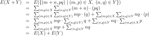 Going from the first to the second line (and the fifth to sixth)
we use the definition of expectation,
and going from the fourth to the fifth we use the fact that the sum of all the
probabilities for any random variable is 1. The rest is properties of
arithmatic, i.e. multiplication and addition distribute over each other.
Now we have completed the goal stated in the first paragraph. If we roll
a dice 100 times then the expected value of the sum of the rolls
is 100E(X) = 350. This would indicate that if the sum of the rolls is
100, then the dice probably isn't fair.
Going from the first to the second line (and the fifth to sixth)
we use the definition of expectation,
and going from the fourth to the fifth we use the fact that the sum of all the
probabilities for any random variable is 1. The rest is properties of
arithmatic, i.e. multiplication and addition distribute over each other.
Now we have completed the goal stated in the first paragraph. If we roll
a dice 100 times then the expected value of the sum of the rolls
is 100E(X) = 350. This would indicate that if the sum of the rolls is
100, then the dice probably isn't fair.
However, this isn't the whole story. For example, if you said you got 50
1's and 50 6's, then the sum would be 350, which is exactly what the
expected value is. We need some other kind of measurement to go along with
the expected value measurement. One candidate is the variance. This
is supposed to measure how different the values are from the average
value, and is defined as  . Notice that in the first
equation we are subtracting E(X) from X. This is the same as adding the
random variable {(-E(X),1)} to X. (E(X) is a constant, because it doesn't
depend on the possible outcomes of X, which we are summing over.) Now when
we square the random variable (X - E(X)) we aren't actually multiplying
two random variables together, we're just squaring the numbers that are the
possible outcomes. More precisely, the square is defined as
. Notice that in the first
equation we are subtracting E(X) from X. This is the same as adding the
random variable {(-E(X),1)} to X. (E(X) is a constant, because it doesn't
depend on the possible outcomes of X, which we are summing over.) Now when
we square the random variable (X - E(X)) we aren't actually multiplying
two random variables together, we're just squaring the numbers that are the
possible outcomes. More precisely, the square is defined as  .
.
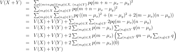
The obvious next question is how does variance interact with addition?
If the random variables are independent (which means that the outcome of one
doesn't depend at all on the outcome of the other), then variance is also
additive, as we show below. Throughout the mu's with the subscript refer
to the expectation of X and Y.
 Plugging into the formula, if X is the random variable corresponding to the
roll of 1 dice, then V(X) = 1/6(2.5^2+1.5^2+.5^2+.5^2+1.5^2+2.5^2) =
3 - 1/12. (Unfortunately it isn't an integer or very nice fraction.)
This gives us another way to test if a sequence of dice rolls is random. If
someone claimed they rolled 50 1's and 50 6's, then the sum of their rolls
would be 350, which is exactly the expected value of the sum of 100 dice
rolls. However, the variance would be 50*(6-3.5)^2 + 50*(1-3.5)^2 = 625,
but the variance of the random variable corresponding to the sum of 100
dice rolls would be 300 - 25/3, or about 292, which is much smaller. Now we
have two ways to tell if a sequence isn't random. Of course, these will
miss some ways that sequences can fail to be random, for example, the
sequence of rolls 1,2,3,4,5,6,1,2,3,4,5,6,... will appear to be random
using these tests. Of course, this sequence of rolls will be impossible to
reject as nonrandom by any test which doesn't depend on the order of the
rolls, since the distribution of the numbers is exactly what it should be.
Plugging into the formula, if X is the random variable corresponding to the
roll of 1 dice, then V(X) = 1/6(2.5^2+1.5^2+.5^2+.5^2+1.5^2+2.5^2) =
3 - 1/12. (Unfortunately it isn't an integer or very nice fraction.)
This gives us another way to test if a sequence of dice rolls is random. If
someone claimed they rolled 50 1's and 50 6's, then the sum of their rolls
would be 350, which is exactly the expected value of the sum of 100 dice
rolls. However, the variance would be 50*(6-3.5)^2 + 50*(1-3.5)^2 = 625,
but the variance of the random variable corresponding to the sum of 100
dice rolls would be 300 - 25/3, or about 292, which is much smaller. Now we
have two ways to tell if a sequence isn't random. Of course, these will
miss some ways that sequences can fail to be random, for example, the
sequence of rolls 1,2,3,4,5,6,1,2,3,4,5,6,... will appear to be random
using these tests. Of course, this sequence of rolls will be impossible to
reject as nonrandom by any test which doesn't depend on the order of the
rolls, since the distribution of the numbers is exactly what it should be.
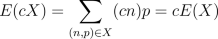
We've talked about addition of random variables, but we haven't talked
about multiplying them by a scalar quantity (this would be like multiplying
the values on a dice by some fixed number). If c is a fixed number
and we write cX to denote this process, then we can figure out what
happens when we take the expectation and variance of cX.
 Therefore, if instead of adding up 100 dice rolls we wanted to average
100 dice rolls, our expectation would remain the same but the variance would
decrease. Specifically, if X_i corresponds to the roll of dice number i,
then
Therefore, if instead of adding up 100 dice rolls we wanted to average
100 dice rolls, our expectation would remain the same but the variance would
decrease. Specifically, if X_i corresponds to the roll of dice number i,
then 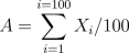 is the average of 100 rolls, and E(A) = 3.5 and
V(A) = (3-1/12)/100.
is the average of 100 rolls, and E(A) = 3.5 and
V(A) = (3-1/12)/100.
In the episode Charlie briefly mentions that dynamic fluid flow equations
(which are PDEs, partial differential equations) can help optimize the
widths of roads, speed limits, etc. in systems of roads. We won't discuss
this here because it involves advanced calculus, but there is an interesting
and un-intuitive fact that we will mention. If you have a system of roads
and then add a road to it, it can actually increase average travel times of
the drivers on the road! A short explanation of why this can happen is as
follows: each driver is trying to minimize his/her total driving time and
doesn't care about the driving times of other drivers. This means he/she
doesn't care about the average driving time very much. Since the only
optimization occuring is the optimization performed by the individual
drivers and they don't care about average driving time, there's no reason
to expect that average driving time will be minimized. This is very similar
to the Prisoner's Dillemma, where the prisoner's
total utility is highest if they cooperate, but if they operate selfishly
they do not achieve this maximum total utility.
One reason the concept of adding random variables is
important is a deep mathematical theorem called the Central Limit Theorem.
The basic idea of this theorem is that the sum of many copies of the same
random variable is approximated very well by the Gaussian Distribution,
or to use plainer English, looks like a Bell curve. This is nice because
the Gaussian distribution has the very nice property that it is completely
determined by its expected value and variance. Furthermore, if we call
the square root of the variance a standard deviation, then if we evaluate
(also called sampling) the Gaussian distribution, 68%, 95% and 99.7%
of the time the
value will be within 1, 2, and 3 standard deviations of the expected value,
respectively. (If X is the random variable corresponding to rolling a dice,
then sampling X means rolling the dice and seeing what the value is.) This
gives us a more quantitative way of declaring that some sequences of rolls
are unlikely to be random. For example, if we roll a dice 20 times, then
then expected average of these rolls will be 3.5 and the variance of the
average will be (3-1/12)/20, which is about .13. Then averages of above
3.63 or below 3.37 will only occur 32% of the time, and averages of above
3.89 or below 3.11 will only occur .3% of the time.
Activity 3:
- Find the expected value and variance of the random variables
corresponding to the sum and average of 20 dice rolls.
- Take the lists from activity 1 and calculate each of the values
in the previous problem for both lists. Which list, the random or
human-generated one, has "better" values (closer to what you expect)?
- Would these tests have helped you to predict which list was random?