| The goal here is to observe the general central limit theorem in computer simulation. |
| ||
I. Simulation Study
LetX be a uniform random variable and let Y be the random variable given by  .
To study the distribution of
.
To study the distribution of Y, first use simulation to generate one DataDesk variable XR containing 200 Realizations of X.
We will refer to this DataDesk variable as YR which contains 200 Realizations of the random variable Y . By default, DataDesk will name it something like  which serves as a reminder of how you arrived at the values in
 YR .
- Computer Hint:
- Generate the Realization of
X,XRusing the menu entry Manip → Generate Random Numbers... Specify1variable with200cases, and select the uniform distribution. - Create the Realizations of
Y,YRfromXR( Manip → Transform → Sqrt(y) ).
- Generate the Realization of
- Plot the histogram of
YR‡ - based on the histogram of
YR, doesYappear to have a uniform distribution? DoesYappear to have a Normal Distribution? Why or why not? Do the heights of the histogram bars generally increase or decrease as the value ofYincreases between0and1? Explain intuitively in terms of the graph of .
.
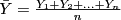
- Based on the simulation study (i.e. using the sample mean ‡ and sample standard deviation ‡ of YR), what is your estimate of the mean of
Yand standard deviation ofY? - The mean and standard deviation of
Yare exactly and
and  respectively. Are the estimates in part (3) close to the exact values?
II. Central Limit Theorem
For the rest of the lab you will be filling in the table below:| n | exact mean | mean(YBAR) (From Simulation) | exact SD | SD(YBAR) (From Simulation) | exact variance | variance(YBAR) (From Simulation) |
| 1 | | |  | |||
| 5 | ||||||
| 10 |  | |||||
| 40 |
 following the same distribution as
 Y above with
 and we want to study the distribution of
  .
.
- Be careful! As you look at each different sample size, be sure to:
- Generate the appropriate number of Uniform Random Variables, x
- Take their Square Roots to arrive at a corresponding number of Random Variables y
- Create a new derived variable for based on the relevant sample size.
- Plot your histogram
- Calculate your summary statistics.
- Write values in the table above.
- For n =
5what are the exact values of the mean and standard deviation of ? For n =
5, generate 200 realizations of. Computer Hint Note this means that you first have to generate 5variables (each has 200 cases) of realizations using the method of Problem I. After you have generated these
 5variables, average them by the following steps: First use the menu entry Data → New → Derived Variable to write a formula. Assign the nameYBARto this variable. If your5variables with the same distribution asYare named , then you'd like to enter
  as the defining formula of the derived variable
 YBAR. A way to do this with less typing is to select the5icons and drag them into the window where YBARis being defined. This will give a list of these variable separated by commas. Now edit the commas, changing them to plus signs. This technique will really help on question III below when we ask you to do this for40variables! An alternative is suggested at the end of the assignment. - Based on your simulation of
YBAR, estimate the mean ‡ and the variance ‡ ofYBAR. How do they compare to the exact values in (1)? - Plot the histogram ‡ of
YBAR. Does the distribution look normal?
III. Larger n
Redo Problem II, for n =10 and n = 40 and fill in the rest of the table above.
( You need to redo all three parts in II for n = 10 and n = 40).
For n = 40, what does the Central Limit Theorem say that the approximate distribution of YBAR is?
What are the mean and standard deviation of this approximating distribution?
Note in selecting 40 icons, you can just use your mouse, starting at the leftmost, and while holding the mouse button down, drag a rectangle touching all 40 icons to be included in the definition of YBAR.
You will have to change 39 commas to plus signs to come up with this informative average. You can do them one at a time in DataDesk, but a better way is to copy and paste into a text editor with search and replace. Do the search and replace and then copy and paste back into DataDesk. Note: When you copy/paste into your text editor, you may find that the √ symbol becomes something else. Don't worry about it. It should return to its original form when pasted back into DataDesk after you have done the replace/copy operation.
Note:
An alternative is to generate200 variables of 40 cases each.
All 200 variables are selected at this point.
Use Manip → Transform →  then Calculate Summaries as Variables.
A new window opens with variables mean, standard deviation, counts, etc.
This depends on the requested summary variables.
Do a histogram of the mean.
This exercise is designed to illustrate ideas from Chapter 18 of Stats Data and Models by DeVeaux, Velleman and Bock.
The density curve of
then Calculate Summaries as Variables.
A new window opens with variables mean, standard deviation, counts, etc.
This depends on the requested summary variables.
Do a histogram of the mean.
This exercise is designed to illustrate ideas from Chapter 18 of Stats Data and Models by DeVeaux, Velleman and Bock.
The density curve of  is
is 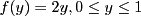 .
.
To Turn in:
- Please print out the results marked with ‡.
- Hand in your completed assignment when your TA asks for it in lab next week..
 → CuMath171Info > LabExercises → LabOnTheCentralLimitTheorem
 Revision: LabOnTheCentralLimitTheorem - r1.15 13 Mar 2007 - 18:43 - Dick Furnas