Spectral Decimation
This page should clarify the concept of spectral decimation on the Sierpinski Gasket.
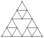
It is extremely difficult to conduct numerical analysis on the Sierpinski Gasket itself because it is infinitely deep. Instead we work on graph approximations of the Gasket. Below are the first three graph approximations for the gasket, on levels 0, 1, and 2. Level 0 has only the boundary points, while level one includes the midpoints of the connecting edges, level two includes the midpints of each smaller edge, etc. We'll designate levels by the letter m.
m=0 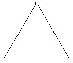 m=1
m=1 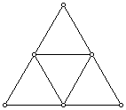 m=2
m=2 
The eigenfunction is across the entire gasket, but we can only approximate the eigenvalue by using a series of graph eigenvalues. As we go to deeper and deeper levels, we find that more and more eigenvalues appear. A good analogy for this is a look at the unit interval. First let's look at something analogous to level 0. This is where you can only see boundary points. Now, let's assign values of 0 to each boundary point. We can see that the equation y1=sin(pi*x) fits nicely. But so do y2 = sin (2*pi*x) and y3 = -sin(3*pi*x). If we move to level 1, which includes the first midpoint, we'll notice an interesting development. y1 and y2 bifurcate into two separate and distinct equations (y1 has value 1 at the midpoint, while y2 is still 0 there). But we still can't tell y3 from y1. To do this we need to go to level 2, which allows us to see y1 bifurcate into itself and y3.
So, although on the entire unit interval it is easy to tell the equations y=sin(pi*k*x) apart, when we use graph approximations the equations appear to bifurcate and distinguish themselves at each subsequent level. This is spectral decimation.
In the case of the Sierpinski Gasket, we have two choices for eigenvalues on each subsequent level, determined by our previous choice. These choices are ruled by the following equation, where epsilon can be either 1 or -1:

The sequence of eigenvalues on graph approximations is what determines the final eigenvalue on the gasket, governed by this equation, where the j represents the particular sequence of pluses and minuses we make.

The ordering of j's corresponds to size, so that the j=1 corresponds to the smallest eigenvalue in that series. There are three series which come into play often, the 2-series, 5-series, and 6-series. The naming of these series follows the value of lambda on the 1st level for the 2-series and 5-series, the 2nd level for the 6 series. One can start the 5-series on any interior triangle as well, making a sort of nested 5-series.
One can only choose epsilon to equal 1 finitely many times, after that, all choices must be -1.
All of my work was done using the first 512 eigenvalues on the 2-series and the 5-series. As it turns out, the normal derivative on the 6-series is 0 everywhere, and thus, pretty uninteresting.
back
main
 m=1
m=1  m=2
m=2 