The Mathieu Differential Equation and Generalizations to Infinite Fractafolds

In this section we give an introduction to the Mathieu differential equation (MDE). A discussion of the relation between the Mathieu equation and fractafolds will be postponed until the next section.

We begin by defining the Mathieu differential equation.

Definition 1 (Mathieu differential equation):
The Mathieu differential equation is given by $$\frac{d^2u}{dx^2}+\left(\delta+\varepsilon\cos x\right)u=0$$ where $\delta,\varepsilon\in\mathbb{R},$ and $u:\mathbb{R}\to\mathbb{R}.$

The Mathieu differential equation (often simply referred to as 'the Mathieu equation') was named for French mathematician Émile Léonard Mathieu (1835-1890). The Mathieu equation as a number of real-world applications, such as to the motion of a pendulum. See chapter 5 of Nonlinear Vibrations in Mechanical and Electrical Systems (Vol. 2 New York: Interscience Publishers, 1950) by James J. Stoker for a further discussion. As discussed in Nonlinear Vibrations in Mechanical and Electrical Systems, the particular values of $\delta$ and $\varepsilon$ one chooses can drastically alter the corresponding solutions to the Mathieu equation. With this in mind, we make the following definition.

Definition 2 (Stable and Unstable Pairs of $\delta$ and $\varepsilon$):
An ordered pair $(\delta,\varepsilon)\in\mathbb{R}^2$ forms a stable pair of values if each solution to the corresponding Mathieu equation remains bounded for all $x\in\mathbb{R}.$ An ordered pair $(\delta,\varepsilon)\in\mathbb{R}^2$ forms an unstable pair of values if there exists a solution to the corresponding Mathieu equation which is unbounded.

From these definitions of stable and unstable $\delta$-$\varepsilon$ pairs, it is natural to wonder if there is a systematic method in which one might about determining which pairs of delta and epsilon are stable and which pairs are unstable. This question has been answered in the affirmative (see Nonlinear Vibrations in Mechanical and Electrical Systems by Stoker for details), and we give a summary of such known results as follows.

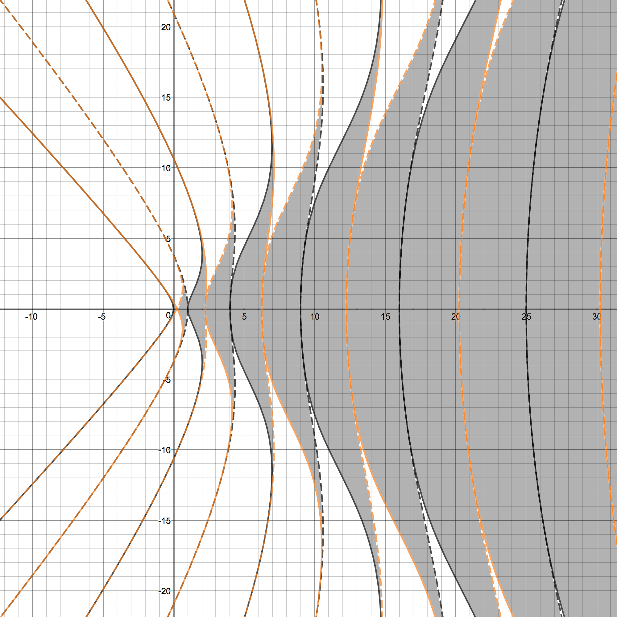
Consider the image below of the $\delta\varepsilon$-plane. In this plot, the horizontal axis is the $\delta$-axis, and the vertical axis is the $\varepsilon$-axis. The shaded region represents regions of the $\delta\varepsilon$-plane corresponding to stable pairs of values, and the white regions correspond to unstable pairs of values. The dark curves that separate these two regions are called the transition curves.

It can be shown that the transition curves for the Mathieu equation share a number of interesting properties. We state below, without proof, some of these properties (see Nonlinear Vibrations in Mechanical and Electrical Systems by Stoker for a further discussion):

• Each transition curve crosses the $\delta$-axis exactly once, and does so at a point of the form $(\delta_n,0),$ where $\delta_n:=\frac{n^2}{4}$ with $n\in\mathbb{N}.$
• To each $\delta_n,$ where $n\geq1,$ there are exactly two transition curves that cross the $\delta$-axis through $\delta_n.$
• The transition curves are symmetric about the $\delta$-axis.
• Each transition curve asymptotes to have slope +1 as $\varepsilon\to\infty$ (and, hence, by the aforementioned symmetry of the transition curves, asymptotes to have slope -1 as $\varepsilon\to-\infty$).
• No two transition curves intersect, except possibly at points of the form $(\delta_n,0).$
• Points on the transition curves where $\varepsilon=0$ are stable, whereas all other points on the transition curves are unstable.

Hence, from this figure it is easy to see that, once one determines where the transition curves lie on the $\delta\varepsilon$-plane, one can determine the stability for all other $(\delta,\varepsilon)$ in the plane since they are, roughly speaking, separated into regions 'between' the transition curves.

Now we consider the main question which is to be addressed in the remainder of this section, which is "How would one actually go about determining, a priori, what the plots of the transition curves, as shown above, look like?". In other words, our aim is to explain a method in which one can obtain the curves shown in the figure. As we shall see, insight into this question can be obtained from the following theorem, which we paraphrase from Nonlinear Vibrations in Mechanical and Electrical Systems.

Theorem 1 (Stoker):
A pair $(\delta,\varepsilon)$ lies on a transition curve for the Mathieu equation if and only if there exists a corresponding nontrivial solution $u:\mathbb{R}\to\mathbb{R}$ which is periodic with period $2\pi$ or $4\pi.$

Hence, if we can determine which pairs $(\delta,\varepsilon)$ yield a periodic solution of period $2\pi$ or $4\pi,$ then we have thus determined the transition curves. (Note, however, that a solution which is $2\pi$-periodic is automatically $4\pi$-periodic. Thus, it suffices to determine which pairs $(\delta,\varepsilon)$ have a corresponding solution of period $2\pi.$)

To this end, let us suppose we have a periodic solution $u(x)$ to the Mathieu equation. In this case, we can write the Fourier expansion of $u$ as $$u(x)=\sum_{k=0}^\infty a_k\cos\left(\frac{2\pi k}{L}x\right)+ \sum_{k=1}^\infty b_k\sin\left(\frac{2\pi k}{L}x\right)$$ where $L$ is the period of $u.$ If we assume $u$ is $2\pi$-periodic, then we would set $L=2\pi$, and if we assume $u$ is $4\pi$-periodic, then we would set $L=4\pi$. However, for the sake of generality, we let $L=2\pi N,$ where $N\in\mathbb{N}$ is arbitrary, in which case our Fourier expansion for $u$ becomes $$u(x)=\sum_{k=0}^\infty a_k\cos\left(\frac{k}{N}x\right)+ \sum_{k=1}^\infty b_k\sin\left(\frac{k}{N}x\right).$$ If we plug this Fourier series for $u$ into the Mathieu equation, rearrange terms, and use some trigonometric identies, we find that the Mathieu equation is equivalent to the combination of the following two infinite systems of linear homogeneous equations for the cosine and sine coefficients, respectively: \begin{matrix} \delta a_0+\frac{\varepsilon}{2}a_N=0\\ \\ (\delta-\lambda_1)a_1+\frac{\varepsilon}{2}(a_{N+1}+a_{N-1})=0\\ (\delta-\lambda_2)a_2+\frac{\varepsilon}{2}(a_{N+2}+a_{N-2})=0\\ (\delta-\lambda_3)a_3+\frac{\varepsilon}{2}(a_{N+3}+a_{N-3})=0\\ \vdots\\ (\delta-\lambda_{N-1})a_{N-1}+\frac{\varepsilon}{2}(a_{N+(N-1)}+a_{N-(N-1)})=0\\ \\ (\delta-\lambda_N)a_N+\frac{\varepsilon}{2}(2a_{0}+a_{2N})=0\\ \\ (\delta-\lambda_k)a_k+\frac{\varepsilon}{2}(a_{k-N}+a_{k+N})=0,\quad(k\geq N+1)\\ \\ \end{matrix} and \begin{matrix} (\delta-\lambda_1)b_1+\frac{\varepsilon}{2}(b_{N+1}-b_{N-1})=0\\ (\delta-\lambda_2)b_2+\frac{\varepsilon}{2}(b_{N+2}-b_{N-2})=0\\ (\delta-\lambda_3)b_3+\frac{\varepsilon}{2}(b_{N+3}-b_{N-3})=0\\ \vdots\\ (\delta-\lambda_{N-1})b_{N-1}+\frac{\varepsilon}{2}(b_{N+(N-1)}-b_{N-(N-1)})=0\\ \\ (\delta-\lambda_N)b_N+\frac{\varepsilon}{2}b_{2N}=0\\ \\ (\delta-\lambda_k)b_k+\frac{\varepsilon}{2}(b_{k-N}+b_{k+N})=0,\quad(k\geq N+1).\\ \end{matrix} Observe that, for any given $\delta$ and $\varepsilon,$ specifying $a_0$ and $a_1$ uniquely determines the values of $a_k$ for all $k\geq2.$ Similarly, for any given $\delta$ and $\varepsilon,$ specifying $b_1$ and $b_2$ uniquely determines the values of $b_k$ for all $k\geq3.$ We can put these two systems of equations into matrix form as follows: \[ \left( \begin{array}{cc} \delta & \frac{\varepsilon}{2} &\\ \varepsilon & \delta-1^2 & \frac{\varepsilon}{2} &\\ & \frac{\varepsilon}{2} & \delta-2^2 & \frac{\varepsilon}{2}\\ & & \frac{\varepsilon}{2} & \delta-3^2 & \frac{\varepsilon}{2}\\ & & & \ddots & \ddots & \ddots \end{array} \right) % \left( \begin{array}{cc} a_0 \\ a_1 \\ a_2 \\ a_3 \\ a_4 \\ \vdots \end{array} \right) = \left( \begin{array}{cc} 0 \\ 0 \\ 0 \\ 0 \\ 0 \\ \vdots \end{array} \right) \] \[ \left( \begin{array}{cc} & \delta-1^2 & \frac{\varepsilon}{2} &\\ & \frac{\varepsilon}{2} & \delta-2^2 & \frac{\varepsilon}{2}\\ & & \frac{\varepsilon}{2} & \delta-3^2 & \frac{\varepsilon}{2}\\ & & & \ddots & \ddots & \ddots \end{array} \right) % \left( \begin{array}{cc} b_0 \\ b_1 \\ b_2 \\ b_3 \\ \vdots \end{array} \right) = \left( \begin{array}{cc} 0 \\ 0 \\ 0 \\ 0 \\ \vdots \end{array} \right). \]

Note that both of these systems consist of infinite matrices.

Now, recall from Theorem 1 above that a pair $(\delta,\varepsilon)$ is on a transition curve for the Mathieu equation if and only if there exists a nontrivial solution $u(x)$ which is periodic with period $2\pi$ or $4\pi.$ (If $u$ is the trivial solution, then $0=a_k$ for all $k\geq0$ and $b_k$ for all $k\geq1,$ in which case $u$ is a solution for any $(\delta,\varepsilon)$ on the $\delta\varepsilon$-plane. Hence, we are not interested in the trivial solution, as it gives no insight into the detmination of which pairs $(\delta,\varepsilon)$ lie on the transition curves). So, we henceforth assume that our solution $u$ to be nontrivial. In finite-dimensional linear algebra, a homogeneous matrix system of equations has a nontrivial solution if and only if its determinint is nonzero. However, since our systems of equations are infinite, our situation is a bit different. However, there is a way around this.

Fix $m\in\mathbb{N}$ and consider the $m\times m$ leading principal submatrix each of our systems. Taking the determinant of this matrix (which is a 'truncation' of our original, infinite matrix) yields an algebraic expression involving $\delta$ and $\varepsilon.$ If we wish that the determinant of this $m\times m$ matrix be nonzero, we simply set this resulting algebraic expression equal to zero. We can then plot this equation in the $\delta\varepsilon$-plane, leading to a set of disjoint curves. If we choose $m$ sufficiently large, then the resulting curves drawn in the $\delta\varepsilon$-plane by setting the determinant of the $m\times m$ leading principal submatrix equal to zero will be a very close approximation to the true curves that arise if one were to consider the curves that result from the case of the infinite matrix. So, this is the approach we take. An example of such an $m\times m$ truncation for the system involving the cosine coefficients (the $a_k$ terms) is shown below. The case for the sine coefficients is similar.

\[ \left( \begin{array}{cc} \delta & \frac{\varepsilon}{2} &\\ \varepsilon & \delta-1^2 & \frac{\varepsilon}{2} &\\ & \frac{\varepsilon}{2} & \delta-2^2 & \frac{\varepsilon}{2}\\ & & \frac{\varepsilon}{2} & \delta-3^2 & \frac{\varepsilon}{2}\\ & & & \ddots & \ddots & \ddots\\ & & & & \frac{\varepsilon}{2} & \delta-(m-1)^2 & \frac{\varepsilon}{2} \end{array} \right) % \left( \begin{array}{cc} a_0 \\ a_1 \\ a_2 \\ a_3 \\ a_4 \\ \vdots \\ a_m \end{array} \right) = \left( \begin{array}{cc} 0 \\ 0 \\ 0 \\ 0 \\ 0 \\ \vdots \\ 0 \end{array} \right) \] 

A complete list of references can be found from our paper on ArXiV.org.