1-Dimensional Maps and Cobweb Dynamics

One-dimensional maps (sometimes called difference equations or iterated maps or recursion relations) are mathematical systems that model a single variable as it evolves over discrete steps in time. As a simple example, start with the number on your calculator and continually press the cosine button.

Assuming that you are using radians as your units, the following series of numbers should appear: , , , , etc. If we label each of the consecutive points , , , and respectively, the sequence of numbers is called the orbit starting from .

One-dimensional maps come from:

1. Modeling natural phenomena such as population dynamics, electronics, economics, etc.
2. Simple examples of chaos.

Consider the system , where where is the current state of the system, is the next state, and is a smooth function (just tells us that satisfies some "nice" properties) mapping the real line to the real line. A point such that is called a fixed point. Why? Consider the system given above and assume that . Then

Therefore the state of the system remains fixed. Thus, to find a fixed point of a given one-dimensional map we just set and solve for . However, there is an easier, graphical way of determining fixed points (and other long-term orbit behavior) via the use of cobweb diagrams.

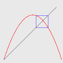
Shown below is an example of a cobweb diagram. The curved line is a plot of the logistic map to be discussed later. The diagonal line is a plot of the curve (we will refer to the vertical axis as the y-axis and the horizontal axis as the x-axis).

The remaining series of lines represents the cobweb. Starting at the right-most point we proceed as follows. We start along the -axis at our initial point . Under the map (which in the above diagram is given by the logistic map) the initial point gets mapped to a new point which we find by drawing a vertical line from the -axis up to the curve representing . To find the next point in the orbit we begin by moving horizontally to the curve . Our x-coordinate will now be . We can now find the next point in our orbit, , by once again drawing a vertical line up (or down) to the curve . We then continue this procedure until we have calculated as many points in the orbit of as we wish.

Another way to view the construction of the cobweb diagram is:

We note that with this graphical construction it is quite easy to find any fixed points of a map. By the definition given previously, a fixed point will occur at a value where the graph of and intersect in the above diagram.

Computer Programs

The following Java programs were authored by Adrian Vajiac and are hosted on Bob Devaney's homepage: http://math.bu.edu/DYSYS/applets/index.html.

The first program we will use is Linear Cobweb Diagrams. This Java program allows the user to construct cobweb diagrams and also graph successive function values for the simplest type of map - a linear function. The program allows one to choose the parameters for the linear function and also an initial value to start iterating with. Complete instructions for the program can be found by clicking on the link entitled "More about Linear Web." By using the program, the students should try to answer the 5 questions posed at the end of the instructions. A short discussion on stability should follow.

To see cobweb diagrams with more complicated functions than just linear, use the Nonlinear Web program. We will go into the behavior of the logistic function and how it depends on the constant much more later, but this program is useful for showing how complicated the long-term behavior of one-dimensional maps can be.

The next program is Target Practice Game. This game turns the task of constructing a cobweb diagram with the logistic map into a game. Students will gain further understanding about the dynamics of a one-dimensional orbit. Once they master the easy level, the students should try the more advanced levels. There's a trick to figuring out where to put the first point (other than trial and error). Can you figure it out?

Periodic Orbits

So far we have seen (via cobweb diagrams) orbits that either decay to or diverge from a fixed point. Another common type of long-term behavior is that of a limit-cycle (also known as an -cycle where represents the period of the orbit). A limit-cycle is an orbit whose motion is periodic (in other words, the orbit eventually evolves to a series of points that repeats itself. The number of iterations it takes to repeat itself is called its period). For example, for a map to have a -cycle (or period- orbit) we would require . Why?

The fourth program is Target Practice Game (Advanced). This game essentially works the same way as the previous game, except now the final targets are periodic orbits. Note that it is nearly impossible to find a periodic orbit exactly in the game, so the game sometimes allows you to win when it appears the cursor is not exactly on the limit cycle.