Introduction to the Logistic Map

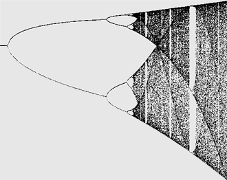
We pick some number between and and fix it. Then we pick any number between and . We let . Then we let , and so on using the rule that . We are interested in studying the long-term behavior of points under iteration of this map, which depends on the parameter . This family of functions is collectively referred to as the logistic map. They are all defined by the equation . In lesson 2, we saw an introduction to the logistic map with Rodin Enchev’s web applet Nonlinear Web, which is an easy way to see visually what the behavior of this map looks like. Another excellent Java program which illustrates long term behavior of this map by Andy Burbanks can be found here.

This equation is a very simple model for animal population in an environment with a limited carrying capacity. The number represents what fraction of the environmental carrying capacity the current population is currently filling up. What the equation says is that the population of a given species after the next time step (which we can take as being the length of a generation of this species) is proportional to two factors. One factor is the number of animals currently alive in the population, , because each individual can only have a limited number of offspring. The other factor is how much carrying capacity is left in the environment, , because if there are too many adults currently alive using up resources then there will be no resources left over for the next generation. So, when one generation of the species is over-populated, that is to say that the population is greater than , then there will actually be fewer animals in the next population. In this view, is a parameter that represents a combination the fecundity and mortality of the population. Higher values of represent a more fertile species which is less likely to die off.

Simple Behavior of the Logistic Map

When is less than or equal to , then no matter what initial starting value for the population we start with, the population will always tend towards in future generations. That is, no population can sustain itself. Using the Nonlinear Web applet, it is easy to see why using the cobweb diagram technique introduced in lesson 2. When is in this range, then the graph of the function is always below the graph of the function , so to iterate the function, we always go down from the line to the graph , and then left again to the line . Iterating the map will always yield a smaller population next generation than there is this generation, and this means that all populations will eventually approach . The following is a cobweb diagram of when is less than :

You can verify algebraically that the intersections of the two graphs and are always and . So these two population values are the only possible fixed points of the map. When is between and , then the second intersection between these two graphs is between and . The importance of the number is that the function achieves its maximum value at . The function is increasing before this maximum, and decreasing afterwards. So when is between and and starts somewhere less than the fixed point , except for , then the population tends towards the fixed point. If instead, starts off somewhere above the fixed point, then the population will get smaller in each future generation. There are two possibilities. One possibility is that the population will get smaller and smaller in each successive generation, but never smaller than the fixed point, in which case it is forced to converge to the fixed point. The other possibility is that at some point, the population goes below the fixed point, in which case the first situation applies. All told, when is between and , then all initial populations with the exceptions of and will converge to a population of . The following is a representative cobweb diagram for between and :

When is at , the attracting fixed point is , which also happens to be the maximum of the logistic map:

Something interesting happens when surpasses . The slope of the function at the fixed point changes from positive to negative at . The iterates will still converge to the fixed point, but they no longer approach from either the positive side or the negative side, as they did when r was between and . Instead, because of the downward slope at the fixed point they flip-flop on alternate sides of the fixed point. The following is a picture of this phenomenon:

Another change in behavior occurs when r becomes greater than . For greater than , the point is still a fixed point, but the slope at this fixed point becomes steeper than . This means that populations close to the fixed point will oscillate back and forth around the fixed point, but they will tend to get farther away from the fixed point on every iteration, as the following diagram shows: