Introduction to Complex Dynamics
In section on one-dimensional maps, we studied the long term behavior of points under the logistic map 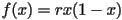 . The family of logistic maps is arguably the simplest family of functions that exhibits such a range of behavior, from extremely ordered and simple actions to more and more complicated behavior to chaos. There is a small extension to the logistic function, which is to allow both
  and
and  to be complex numbers, instead of limiting them to be real. There is a change of coordinates to put all complex quadratic maps into the normal form of
  , where
  is some complex parameter.
The map also has a geometric interpretation. Complex numbers can be naturally described in polar coordinates. Squaring a complex number has the effect of squaring that number's radius (or modulus) and doubling that number's angle (or argument). So squaring the entire complex plane of wrapping the plane twice around the origin. A loop that wraps once around the origin will get mapped to a loop that wraps twice around the origin. So the net effect of the map is to wrap the complex plane around itself and to shift it by some amount .
Another thing that makes this map so interesting to study, apart from its apparent simplicity juxtaposed against the chaos it displays, is the fact that high iterates of most other complex functions begin to look locally like a wrapping around a point along with a translation. So studying this map, the simplest nontrivial map of the complex numbers, can help us understand a wide variety of other functions on the complex plane.
Dynamical Properties
So what can happen to points as we iterate on them repeatedly?
If  gets very large in absolute value, then
  will be tremendously larger, and adding a constant won't make much of an impact, so
  will be even larger than . This means that once points become large enough, then they always escape to infinity.
The complex map has periodic orbits just like its real-valued counterpart, the logistic map, does. Just as in the real case, it is possible for iterates of a point to converge to this periodic orbit.
It is also possible for points to neither escape to infinity nor converge to a periodic orbit. These points bounce around a bounded region of the plane close to the origin, but do so in a chaotic way, never repeating the same patterns.
Julia Sets
One way to visualize the dynamics of the map on the plane is to color points in the complex plane based on whether they escape to infinity or stay in a bounded region for all time. We can color points in the complex plane based on what their long-term behavior is. We can color points that stay bounded one color, and color the points that escape based on how quickly they escape. Here, we will color the points that do no escape black, but other programs may color them differently. The set of points that do not escape is called the filled Julia set, and the boundary of the filled Julia set is called the Julia set. Because of the fact that far enough away from the origin of the complex plane, points always escape, we know that everything of interest is happening in a small region around the origin, and this is all that is usually drawn.
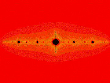
If we let  , then our equation becomes
  . From what we said earlier, each iteration of this function squares the radius of the point being iterated. So points with a radius above 1 will always get larger in absolute value. Points with a radius less than
  will get smaller in absolute value and closer to 0, a fixed point of this map. All future iterates of points with a radius of exactly 1 will also have a radius of exactly , because
  , and they will stay on the unit circle around the origin. The following is a picture of the filled Julia set for :
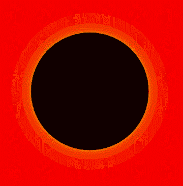
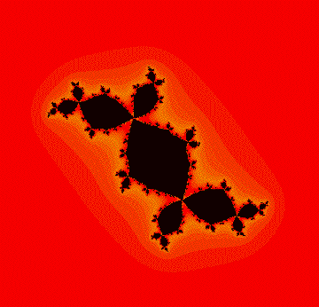
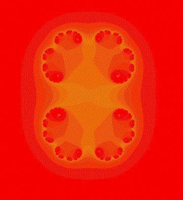
Here are some other pictures of filled Julia sets of maps with other values of . This one is called the Basilica, and occurs when  :
:
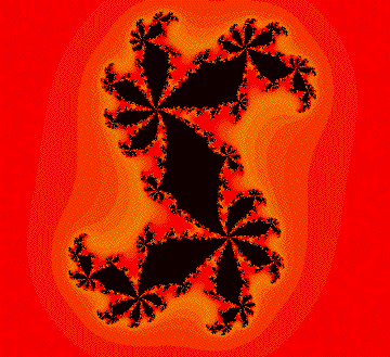
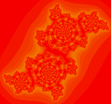
Adrian Douady named the following Julia set the Rabbit because of its prominent ears. 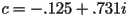 in this picture:
In this picture, 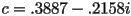
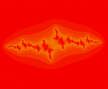
This one is commonly called the airplane, and is achieved when c = -1.755
The previous few examples are relatively simple examples of Julia sets. In all of these examples, the points that do no escape (the black region) is clearly identifiable, and moreover, while it may not be obvious in some of the pictures, the filled Julia set is connected. This does not always have to be the case. The following pictures show filled Julia sets that are not connected. The actual filled Julia sets in these pictures is too small to be seen, but it is there. It’s like a dust that has been sprinkled on the plane, but you can tell where it should be by the coloring of the points based on how long it takes them to escape to infinity. As you move closer and closer to the filled Julia set, the points take longer and longer to escape.
In a sense, each of these filled Julia sets that is not connected is similar to the Cantor Middle Thirds Set. Technically speaking, they are homeomorphic, which just means that in a broad sense, they have the same shape. This quality is not just true for these three examples. Whenever a Julia set is not connected, then it must be simply a collection of dust on the plane, with the same general structure as the Cantor set.
Connected and Disconnected Julia Sets
Julia sets are always either connected or completely disconnected. The reason for this dichotomy is not too hard to see. If a point escapes to infinity, then so do all of its future iterates, and also all of its inverse images. So if the Julia set is disconnected, then we can draw two loops around regions of the Julia set that together contain all of the Julia set, but do not intersect each other. If we take the inverse image of these two loops, then because every point has two inverse images under the function we get four smaller loops, with two of these loops contained in each of the original two loops. Now, we know that the Julia set can be split up into four distinct smaller parts. We can do this procedure over again to show that the Julia set can be split up into eight even smaller parts. We repeat this indefinitely to show that it must be a Cantor set. So a Julia set is either connected or completely disconnected.
There is even an easy way to tell which one of these two possibilities occurs for a particular parameter value. When the point  escapes to infinity, then the Julia set is a Cantor set, but if stays bounded under iteration of the map for all time, then the Julia set must be connected.
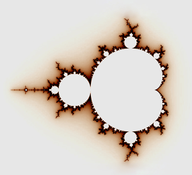
The Mandelbrot Set
Since the behavior of the point has such dramatic implication, it makes sense to track its iteration as a function of the parameter . This is the same question as asking is the Julia set connected or a Cantor set for different values of . The set of all complex values of for which the point does not escape to infinity under iteration of the function is called the Mandelbrot set, and it is of course the same as the set of all values of for which the Julia set of the function is connected.
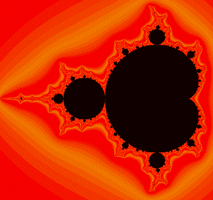
The following is a picture of the Mandelbrot set colored in black. The points not in the Mandelbrot set are colored according to how quickly the point escapes from a bounded region. As approaches the Mandelbrot set, it takes longer and longer for to escape.
Zooming in on parts of the Mandelbrot set can yield shockingly beautiful pictures. There are smaller copies of the entire Mandelbrot set embedded in the boundary, like this one, found near the top of the original :
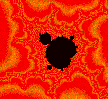
In fact, these smaller copies are dense in the boundary of the Mandelbrot set, which means that anytime you’re looking at part of the boundary, then if you zoomed in more, you would find smaller copies of the entire Mandelbrot set.
Activity - Exploring the Mandelbrot Set
FractInt is a very good program for the PC for looking deeply into the Mandelbrot set. There is a Mac port available as well, though it is still under development. Also for the Mac is FractalAsm, an excellent program for exploring a variety of one complex dimensional dynamical systems written by Karl Papadantonakis. There are also myriad java programs available online. Good ones are here and here. Students can use these programs both to explore Julia sets and the Mandelbrot set and also to explore the relationship between the location of parameter values in the Mandelbrot set and the shape of the Julia sets near there. Julia sets obtained from parameter values near the edge of the Mandelbrot tend to look like the Mandelbrot set does locally near that point. Why?