Families of Risky Assets

Markets are usually diverse and a large amount of assets can be traded (see tangent). In the present lesson we will extend the theory previously developed to markets with more than one risky asset. Implicitly this extension was already considered when explaining the pricing theory of contingent claims in the binomial model. The fair price of a contingent claim was defined so that the extended market, in which the claim is traded, is arbitrage free. In this section we will make this statement more precise and also clarify how prices of European type contingent claims at intermediate times are defined.

Assume that the interest rate in the US is 5%. Suppose for now, that you can borrow and lend Euro and British Pounds with no interest rate. In the diagram below we give the risky exchange rates of the Dollar against the Euro (red) and British Pound (blue) for today and tomorrow. The branches of the tree can occur with equal probability of 0.5 and correspond to the two states of the world, when the exchange rates go up and down, respectively.. Along each of the branches we have placed the corresponding rates of return.

The theory developed in the first module guarantees that in this market there does not exist an arbitrage opportunity that trades only Dollars and Euro or only Dollars and British Pounds, because the interest rate, r, is strictly between the high and low rates of return in each case. However, one might ask, is there an arbitrage opportunity that trades on the three currencies simultaneously? The answer to this question is affirmative. An example of such an opportunity is the following: short-sell €1, borrow $0.1 and buy ₤1. The dollar value today of this strategy is $-1.5-0.1+1.6=$0. The possible values of the portfolio tomorrow are given in the digram below. Each branch in the tree occurs with the same probability of 0.5.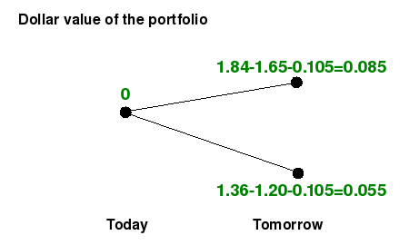

We observe that this strategy represents an arbitrage opportunity: regardless the state of the world, this strategy guarantees positive profits.

Activity 1

Assume that the British Pound's interest rate is 0%, but the Euro's interest rate is 5% (see previous lesson). Explain why the strategy presented above is no longer an arbitrage opportunity in this case.

This example shows that testing for the existence of arbitrage opportunities in a general multi-asset model by just using the definition can become a very complicated problem. Luckily for this end, we can extend the previous theory and use the Fundamental Theorem of Asset Pricing in multi-asset markets as stated below.

The model presented here is a one factor model in the following sense. At each time, there are only two possible movements in the market prices, either all of them jump up or all of them jump down simultaneously. The reason why it is called a one factor model is that the probability of each event occurring can be determined by just flipping one and only one coin. Multi-factors models will be briefly described in lesson 11.

We generalize the model presented in module 1 as follows. Suppose that the market consists of a riskless asset with price process S_t⁰=(1+r)^t and N risky assets with price processes S¹,...,S^N. Assume further that after each time t the price processes jump from S_t¹,...,S_t^N to either S_t+1¹=(1+u¹)S_t¹,...,S_t+1^N=(1+u^N)S_t^N or S_t+1¹=(1+d¹)S_t¹,...,S_t+1^N=(1+d^N)S_t^N, each of these events occurs with positive probability and d^j < u^j for all j between 1 and N (see tangent). This multi-asset model is arbitrage free if an only if

In our example above, we have that r=0.05, d^€=-0.2, u^€=0.1, d^₤=-0.15 and u^₤=0.15. Then

and the model is not arbitrage free (we exhibited an example of an arbitrage opportunity above). It is important to point out that this theorem states that the model is arbitrage free if and only if there exists a probability under which all the discounted risky assets are simultaneously martingales (see lesson 3).

Activity 2

1. Explain why the model of activity 1 above is arbitrage free. Fixing r=0.05, find conditions on the interests rates for the Euro and British Pound for which the model is arbitrage free (see previous lesson).
2. Suppose that General Motors (GM) stock's price behaves as in example 3 of lesson 2. Assume that Ford Motor Company (F) stock's price has rates of return of either 2% when GM stock's price goes up or -2% when GM stock's price goes down. If the dollar's interest rate is 0%, is the market in which GM and F stock are traded arbitrage free?

As mentioned in the beginning of the lesson the fundamental theorem of asset pricing for multi-asset markets clarifies the pricing theory of contingent claims in the binomial model. According to the theorem, if the contingent claim with terminal payoff C is traded at intermediate times between present time and maturity time, the prices of the claim at intermediate times have to be such that the discounted price process is a martingale with respect to the probability q^*. Since at maturity time the price of the claim is equal to its payoff C, we conclude that at time t the price of the claim is

For instance, consider the example given in lesson 4. In this case the possible prices of the call option on the GM stock with maturity date T=2 and strike price 10*0.97 at time t=1 are either

if the price of the stock increases the first day, or

if the price of the stock decreases the first day. We observe that the price of the option is higher when the stock price increases than when it decreases, which makes perfect sense by the definition of a call option.

Activity 3

1. Verify that in the example above the rates of return of the stock and the call option satisfy the condition given in the fundamental theorem of asset pricing for multi-asset models.
2. Find the prices at all times of a put option on the GM stock, with maturity T=2 and strike price of K=10*0.97.