Arbitrage opportunities

In the previous lesson we presented in Example 2 a binomial market where it is possible to find an investment strategy that yields a positive profit with positive probability but without any downside risk. Such a strategy is commonly known as an arbitrage opportunity.

Before giving a formal definition of an arbitrage opportunity it is important to introduce some notation to clarify the concepts of trading strategy and most importantly self-financing trading strategy. A trading strategy is a process that for any time t specifies the quantity of shares in the money market account S⁰ (in our examples this corresponds to the amount of money in dollar currency) and the number of shares of the risky asset S held by the investor between times t-1 and t. We use the following notation for a trading strategy:

It is important to notice that x_t and y_t could take negative values which corresponds to borrowing money and short selling the risky asset, respectively. For instance the strategy presented in Example 2 could be written as x₁=1.5 and y₁=-1.

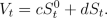
With this notation y_tS_t-1 is the amount invested into the risky asset at time t-1, while y_tS_t is the resulting value at time t. We define the value of the portfolio (c,d) at time t, by

The term arbitrage is commonly referred to as the practice of taking advantage of the price differential between two markets by buying and selling assets. This section is mainly dedicated to making this statement precise. A market with asset prices that rule out these practices is called an arbitrage-free market. An investor that is engaged in an arbitrage opportunity is called an arbitrageur.

We will have a self-financing trading strategy if for any t greater than or equal to 1 and less than or equal to T-1, the value of the portfolios (x_t, y_t) and (x_t+1, y_t+1) at time t are the same. By the observation made in the beginning of the paragraph, this is equivalent to say that the fluctuations in the value of the portfolio are equal to the gains and losses resulting from asset pricing fluctuations only, i.e. there are no cash flows coming in or out.

We define formally an arbitrage opportunity (see Tangent) as a self-financing trading strategy (x,y) such that the value of the initial portfolio (x₁,y₁) at time 0 is less than or equal to 0, but the value of the final portfolio (x_T,y_T) at time T is nonnegative with probability 1 and positive with positive probability.

In order to clarify the concepts and notation introduced above we present some examples.

Example 2 (continued)

The strategy presented in the previous lesson corresponds to x₁=1.5 and y₁=-1. Since we are facing a 1 period model the self-financing condition trivially holds. Observe that the value of the portfolio (x₁,y₁) at time 0 is

However, the value of the same portfolio at time 1 is either 1.5*1.1+(-1)*1.65=0 with probability 0.5 (i.e. if the Euro goes up) or 1.5*1.1+(-1)*1.2=0.45 with the same probability (i.e. if the Euro goes down). This is an example of an arbitrage opportunity in a one step binomial market. We say in this case that the market is not arbitrage-free.

Example 3

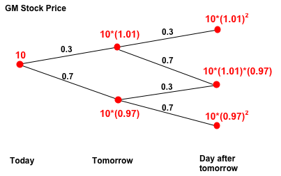
Suppose that today the price per share of Stock for General Motors Corp. (GM) is 10. For the next two days the rate of return is either 1% with probability 0.3 or -3% with probability 0.7. Suppose further that the rate of interest in the money market is 2%. We claim that this binomial market is not arbitrage-free. Consider the following trading strategy, (x,y) x₁=x₂^u=x₂^d=10, y₁=y₂^u=y₂^d=-1, where (x₂^u,y₂^u) and (x₂^d,x₂^d) are the portfolios when the price of the stock after the first day goes up and down, respectively. Since the portfolio does not change at any time this trading strategy is trivially self-financing. At time 0 the value of the portfolio (x₁, y₁) is 10*1+(-1)*10=0. If the price of the stock goes up on day 1 and day 2 then the value of the final portfolio (x₂^u,y₂^u) is equal to 10*(1.02)²+(-1)*10*(1.01)²=0.203. This event occurs with probability 0.3*0.3=0.09 (see Probability Review). If the price of the stock goes down one day but up the other day the value of the final portfolio (x₂^u,y₂^u) or (x₂^d,y₂^d) is equal to 10*(1.02)²+(-1)*10*(1.01)*(0.97)=0.607. Each of these events occurs with probability 0.3*0.7=0.21. Finally, if the price of the stock goes down on day 1 and day 2 the value of the final portfolio (x₂^d,y₂^d) is equal to 10*(1.02)²+(-1)*10*(0.97)²=0.995 This event occurs with probability 0.7*0.7=0.49. Hence, regardless what occurs during these two days the value of the final portfolio is positive and this trading strategy is an arbitrage opportunity. This is an example of a 2 step binomial market that is not arbitrage-free.

Note on self-financing strategies

So far in our examples the self-financing condition holds trivially. In order to better understand the concept, consider the market described in the previous Example and suppose that at time 0 the investor short sells one share of stock (i.e. borrows one share of stock from the broker). At time 1, if the price goes down he pays the stock back to the broker and buys one share in the market, and if the price goes up he does nothing. With our notation the strategy on the stock can be written as x₁=10, y₁=-1, y₂^u=-1, y₂^d=1. Intuitively in order to have a self-financing strategy, the strategy on the money account should balance off the fact that between times 1 and 2 the investor paid back stock to the broker and bought new stock in the market. Formally with the notation developed we have to find x₂^u and x₂^d such that the following holds

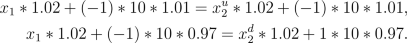
We notice that x₂^u=x₁=10 and x₂^d=x₁+(-2)*(10)*(0.97)/(1.02) is the unique solution to the system above.

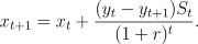
The reasoning above can be generalized and summarized by the following observation. Given any initial portfolio (x₁, y₁) and any strategy on the risky asset S, y₂, ..., y_T, there exists a unique strategy on the money market, x₂, ..., x_T, such that the trading strategy (x,y) is self-financing. This strategy can be found by successive use of the following formula

Activities

Consider the market described in Example 3 but assume that the interest rate r=0. Given an arbitrary initial portfolio (x₁, y₁) and an arbitrary strategy on the risky asset S, y₂, find a strategy on the money market, x₂, such that the trading strategy (x,y) is self-financing.
Hint: Recall that you have to consider two market states, one when the price of the stock goes up the first day and the other one when the price goes down. Hence, your strategy on the money market corresponds to two variables x₂^d and x₂^u which should be given in terms of x₁, y₁, y₂^d, y₂^u.
For the strategy found in part a), write down explicitly the value of the initial portfolio and the possible values of the final portfolios in terms of x₁, y₁, y₂^d, y₂^u.
Explain why it is impossible to find x₁, y₁, y₂^d, y₂^u such that the value of the initial portfolio is nonpositive but the value of the final portfolio is always nonegative and positive at least once. In other words, explain why this market is arbitrage-free.
Hint: In order to prove this you will have to consider a system of inequalities and explain why it is not consitent, i.e. why there are no values of x₁, y₁, y₂^d, y₂^u that satisfy all the inequalities at the same time. At least one of the inequalities should be strict; this corresponds to the fact that in an arbitrage the value of the final portfolio is positive for at least one market state.