The federal fund rate is the interest rate at which depository institutions (typically banks) lend money to other depository institutions over night. With the aim at regulating the supply of money in the U.S. economy, the Federal Open Market Committee (FOMC) periodically sets a target for the federal fund rate, which is then determined by open market.

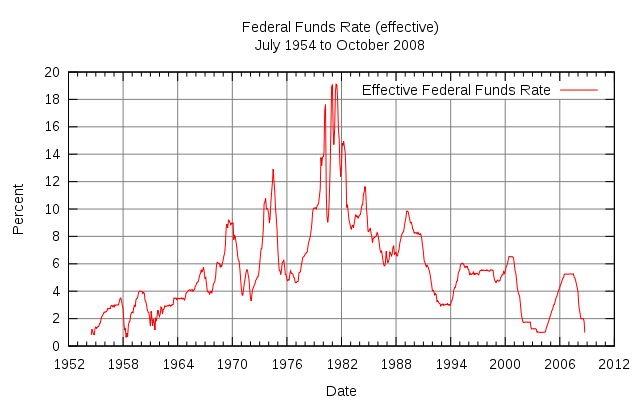
In the multi-period model considered in module 1 we assumed that the interest rate r and the rates of return d and u were constant over time. When trading bonds, the main source of risk in the market comes from the changes over time on the spot interest rate r, and hence is not very accurate to assume this rate to be constant over time. Over long periods of time, even in the stock market, the assumption of constant interest rates might be too restrictive (the figure below shows the federal fund rates between July of 1954 and October of 2008, see tangent). Additionally, when looking at price movements in the stock market it becomes clear that the rates of return over time can not be modeled by just using the two variables d and u. In the present lesson we will restate the fundamental theorem of asset pricing for time dependent interest rates and rates of return. This extension appears to be very simple by it turns out to be very useful, since more robust models can be used in this framework. 

Suppose that the exchange rate of the Euro against the dollar is as in the multi-period model presented in lesson 1. Assume that today the interest rate on the Dollar is 5%, but tomorrow it changes to 10% (see figure below). Assume further that the interest rate on the Euro is 0% for the next two days. By the considerations made in module 1 we know that this model is arbitrage free for the first period of time. One might ask then: is this model, in which interest rates on the dollar depend on time, arbitrage free over the two days time horizon as well?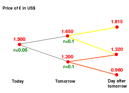

The answer to this question is negative because the interest rate in the second period is not strictly between the rates of return u=0.1 and d=-0.2. An example of an arbitrage opportunity is the following: do not trade today, wait until tomorrow to short-sell €1 and lend the selling price in dollars. This strategy represents an arbitrage opportunity, the value of the strategy at different times is given in the diagram below.

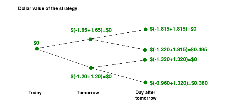
This example illustrates the following fact: a market model is arbitrage free if and only if every one step submodel is arbitrage free as well. In the case above, the one-step submodels obtained when the price goes either up or down (highlighted with yellow and orange in the figure above) are not arbitrage free and neither is the two-step model.

Activity 1

1. Suppose that the stock's price of General Motors is as in lesson 2. Assume that the dollar's interest rate today is 0%, but tomorrow it is 1%. Determine if this market is arbitrage free. In case it is not, give an example of an arbitrage opportunity.
2. Suppose now that the stock pays 1% of dividend on each dollar invested between tomorrow and the day after tomorrow (see lesson 7). Is in this case the market arbitrage free?

As we already mentioned above in order to guarantee the nonexistence of an arbitrage opportunity in a multi-step model it is necessary and sufficient to guarantee the arbitrage free condition over the one-step submodels. This results applies not only when interest rates change over time, as we saw in the example presented above, but also when the rates of return on the risky asset are time dependent as well. In general, if we have a model with a riskless asset with time dependent interest rate r_t and price process S_t⁰=(1+r_t)^t, and a risky asset with time dependent rates of return, d_t< u_t, each of which can be realized at any time with positive probability, and price process S_t, the market is arbitrage-free if and only if at any time t

which holds if and only if the discounted price process

is a martingale with respect to the risk neutral probability, that at each time t gives the probability (r_t-d_t)/(u_t-d_t) to the realization of the rate of return u_t. A natural generalization of this result can be obtained for multi-asset markets (see lesson 8). The statement of this generalizatation is left as an exercise for the reader. Also notice that the result above allows us to study models in which dividend payments on the risky asset are not paid at each time (see lesson 7). For instance assume that in the example above the interest rate on the Euro is 0% today but 10% tomorrow. This pushes up the rates of return on the Euro tomorrow, from d₁=-0.2 and u₁=0.1, to d'₁=-0.12u'₁=0.21 (see lesson 7). Therefore the arbitrage condition of the fundamental theorem is satisfied and the model is arbitrage free (observe that the strategy exhibited above is no longer an arbitrage opportunity under this circumstances).

Activity 2

1. Verify your answer in part b) of activity 1 by using the fundamental theorem for time dependent interest rates and rates of return.
2. Generalize the fundamental theorem for time dependent interest rates and rates of return, when there is more than one risky asset in the market (see lesson 8).

The theorem stated above also reveals how to price contingent claims in models with time dependent interest rate and rates of return. According to the fundamental theorem, the price at time t of a contingent claim with payoff CT at maturity time T is equal to

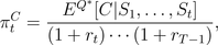
where Q^* is the probability, that at each time t gives the probability (r_t-d_t)/(u_t-d_t) to the realization of the rate of return u_t. For instance, suppose that the stock of GM behaves as in lesson 2, the interest rate over time is given by r₀=0 and r₁=0.01. Assume further that GM pays $1.01 for each dollar invested in the stock between tomorrow and the day after tomorrow. In this case the rates of return are d₀=-0.03, u₀=0.01, d₁=-0.0203 and u₁=0.0201 (see lesson 7). The risk neutral probabilities of the high rates of return today and tomorrow are (0+0.03)/(0.01+0.03)=0.75 and (0.01+0.0203)/(0.0201+0.0203)=0.75, respectively. In this case the price today of a European call option with maturity the day after tomorrow and strike 10*0.97 is

Activity 3

1. Find the prices tomorrow of the call option described above (see lesson 8).
2. Consider the same model as in the example above. Find today's price of a straddle on the GM stock.