In the previous lesson we mentioned that Financial Derivatives are instruments used by investors to reduce the risk in the market. In this lesson we make this statement more clear through some examples. Before reading the material of this section it is recommended to review the notation and concepts of the arbitrage opportunities lesson.

Example 4

Suppose that an investor is facing the market described in the last part of the previous lesson. In this market, under the risk-neutral probability measure, the price of the stock is more likely to go up than down. Call options on the stock reduce the risk of an investor who wants to buy in two days, since it is very likely that the price in two days is going to be higher. As we saw for a strike price of 10*0.97 the price of the call option with maturity of two days is 0.3181875 Now you can imagine that the seller of the call option would be interested in having a strategy to cover the call option. One simple possibility comes from the put-call parity and corresponds to buying a forward contract with the same forward price and a European put option with the same strike and maturity. Another less simple alternative corresponds to finding a strategy in the money market account and risky asset. In this case the seller wants to find a self-financing strategy (x,y) such that the value of the final portfolio is equal to the payoff of the call option. In order to find such a strategy he will have to solve the following system of linear equations

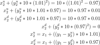
The last two equations account for the self-financing condition (see last note in arbitrage opportunities). The unique solution to this system is approximately x₁=-7.8631, y₁=0.8181, x₂^d=-2.3523, y₂^d=0.25, x₂^u=-9.7, y₂^u=1. Since in this case the system of equations has an exact solution we call the trading strategy (x,y) a perfect hedge or replicating strategy for a European call option with maturity of two days and strike 10*0.97. Observe that the initial portfolio corresponds to borrowing approximately 7.8631 in money and buying 0.8181 shares of the stock. The value of this initial portfolio is approximately 0.32, the price of the European call option. This is not a coincidence and can be generalized for any perfect hedge.

Proposition

If the self-financing portfolio (x,y) is a perfect hedge of a contingent claim with final payoff C, the value of the initial portfolio (x₁,y₁) is equal to the arbitrage free price of the claim, E^Q*[C/(1+r)^T]. Here, Q^* is any risk-neutral probability measure.

Note

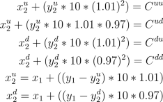
The procedure described in Example 4 above shows how to hedge or replicate a European call option with maturity of 2 days and strike equal to 10*0.97 by using the money market account and the risky asset. This method can be generalized to any contingent claim and in particular to any Financial Derivative. Let C^uu, C^du, C^ud and C^dd be the payoffs when the price goes up both of the days, goes up the first day and down the second day, goes down the first day and up the second day and goes down both days, respectively. Then finding a perfect hedge, (x,y) for this claim corresponds to solving the following system of six linear equations with six unknowns, x₁, y₁, x₂^d, y₂^d, x₂^u, y₂^u,

It is a known result of linear algebra that if a system like this has a unique solution for some values of C^uu, C^du, C^ud and C^dd then it has a solution for any C^uu, C^du, C^ud and C^dd. Hence, since we could find a perfect hedge for a European call option we can find a pefect hedge for any contingent claim. When the latter holds we say that the market consisting of the money market account and the risky asset is a Complete Market. In our model the market completeness is an immediate consequence of the fact that the risk-netral measure Q^* is unique and the following theorem.

The Second Fundamental Theorem of Asset Pricing

A market is complete, i.e any contingent claim can be perfectly hedged, if and only if, there exists a unique risk-neutral probability measure in the market.

Further Analysis

Up to this point we have seen the conditions under which the CRR model with only one risky asset is arbitrage-free. We saw that if these conditions are satisfied then the market is complete and the arbitrage-free price of any contingent claim is the value of the initial portfolio of any replicating strategy or perfect hedge. All this questions become more interesting when we modify our assumptions and we allow more than one risky asset in the market, more than two rates of return at any time and we put constraints to the self-financing strategies, e.g. if short-selling is not allowed or is bounded below by a fix quantity. This elucidates the level of complexity reached by Financial Markets from the mathematical point of view.