A first version of this
theorem was proven by M. Harrison and D. Kreps in 1979. More general
versions of the theorem
were proven in 1981 by M. Harrison and S. Pliska and in 1994 by F.
Delbaen and W. Schachermayer. For these
extensions the condition of no arbitrage turns out to be too narrow and
has to
be replaced by a stronger assumption.
As we have seen in the previous lesson, proving that a market is
arbitrage-free may be very tedious, even under very simple
circumstances.
In this lesson we will present the first fundamental theorem of asset
pricing, a result that provides an alternative way to test the
existence of
arbitrage opportunities in a given market. When applied to binomial
markets, this theorem gives a very precise condition that is extremely
easy to verify (see Tangent).
Before stating the theorem it is important to
introduce the concept of a Martingale.
In simple words a martingale is a process
that models a fair game. To make this statement
precise we first review the concepts of conditional probability and
conditional expectation.
Note
We define in this section the concepts of conditional probability,
conditional expectation and martingale for random quantities or
processes that can only take a finite
number of values. This turns out to be enough for our purposes because
in our examples at any given time
t we have only a
finite number of possible prices for the risky asset (how many?). In
more general circumstances the definition of these concepts would
require some knowledge of measure-theoretic probability theory.
- Conditional Probability
- Given two events A and B
such that P(A) (the probability of A)
is not 0, the conditional probability
of B given A is defined by
-
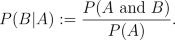
- This
probability
is interpreted as the probability of B given that A
has occured. If the events A and B
are independent we have that P(B|A)=P(B). For
instance, in Example
3 of the previous lesson we have that the probability that
the price of the stock goes up the second day given that it went down
the first day is equal to P(price goes up the second day)=0.3.
- Conditional Expectation
- Once we have defined conditional probability
the definition of conditional expectation comes naturally from the
definition of expectation (see Probability
review). Given a random variable or quantity X
that can only assume the values x1, x2,
..., xn with possitive probability and
an event A such that P(A) is
not 0, the conditional expectation of X given A
under the probability P is

- For instance in Example
3 of the previous lesson we have that
- EP (S2|S1
= 10*0.97)
= 10*0.97*1.01P(S2 = 10*0.97*1.01|S1
= 10*0.97) + 10*(0.97)2P(S2
= 10*(0.97)2|S1 =
10*0.97)
=
10*0.97*1.01*0.3 + 10*(0.97)2*0.7
= 9.5254.
- Martingale
- A random process X0,
X1, ..., XT,
such that for every t between 0 and T,
Xt can only
assume finitely many values xt1,
..., xtnt,
is said to be a Martingale with respect to the
probability measure P if
-

- for all s and i0,
..., is. In other words the
expectation under P of the final outcome XT
given the outcomes up to time s is exactly the
value at time s.
This happens if and only if for any t

Activity 1:
- Suppose Xt
is a gambler's fortune after t
tosses of a "fair" coin (i.e P(heads)=P(tails)=0.5),
where the gambler wins $1 if the coin comes up heads and loses $1 if
the coin comes up tails. By using the definitions above prove that X
is a martingale. This is also known as D'Alembert system and it is the
simplest example of a martingale. It justifies the assertion made in
the beginning of the section where we claimed that a martingale models
a fair game.
- Consider the market
described in Example
3 of the previous lesson. Is the price process of the stock a
martingale under the given probability?
The Fundamental Theorem
A financial market with time horizon
T and price
processes of the risky asset and riskless bond given by
S1,
..., ST and
S10,
..., ST0,
respectively, is arbitrage-free under the probability
P
if and only if there exists another probability measure
Q
such that
- For any
event A, P(A)=0 if and only if Q(A)=0.
We say in this case that P and Q are equivalent
probability measures.
- The discounted
price process,
X0:=S0/S00,
..., XT:=ST/S0T
is a martingale under Q.
A measure
Q that satisifies (i) and (ii) is known
as a
risk neutral measure. After
stating the theorem there are a few remarks that should be made in
order to clarify its content. The first of the conditions, namely that
the two probability measures have to be equivalent, is explained by the
fact that the concept of arbitrage as defined in the previous lesson
depends only on events that have or do not have measure 0. More
specifically, an arbitrage opportunity is a self-finacing trading
strategy such that the
probability that the value of the
final portfolio is negative is zero and the
probability
that it is positive is not 0, and we are not really concerned
about the exact probability of this last event.
Also notice that in the second condition we are not requiring the price
process of the risky asset to be a martingale (i.e a fair game) but the
discounted price process. This can be
explained by the following reasoning: suppose that the price of the
risky asset is measured in dollars. If at time
t
the price of the risky asset is $x, the fair price the seller should
charge at time 0 for the asset should be $x/(1+r)
t,
with r the interest rate. If he charges $y<$x/(1+r)
t
then the buyer could take advantage of the situation by borrowing $y at
time 0 to buy the asset and then selling at time
t
to repay his debt of $y(1+r)
t, obtaining a
positive profit of $(x-y(1+r)
t). If he charges
$y>$x/(1+r)
t then he could take advange
of the situation by selling the asset at time 0 and lending $y dollars
so that at time
t he would receive $y(1+r)
t
and after buying back the asset he would make a positive profit of
$(y(1+r)
t-x). Basically when one considers the
discounted price process every price is being measured in the unity of
the riskless asset
S0, which
is also commonly known in the literature as the
Numéraire.
Activity 2:
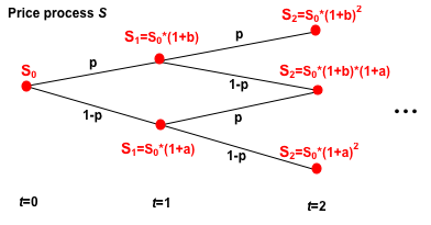
Application of the FFTAP to the CRR Model
Consider a
CRR
Model with interest rate
r. Assume that
at any time
t the return rate of the risky asset
R
satisifes
P(Rt=b)=p and
P(Rt=a)=1-p
with p
strictly greater than 0 and
strictly
less than 1. A binary tree structure of the price process of
the risly asset is shown below.
- Explain why a probability
measure Q such that at
any time t the return rate of the risky asset, R,
satisifes Q(Rt=b)=q and Q(Rt=a)=1-q
and Rt+1,Rt
are independent, is equivalent to P if and only if q
is strictly between 0 and 1.
- Suppose that your time horizon
is T=1 and that Q*
is a measure. Prove that the discounted price process is a martingale
under Q* if and only if at
any time t the return rate of the risky asset R
satisifes Q*(Rt=b)=(r-a)/(b-a)
and Q*(Rt=a)=(b-r)/(b-a).
- Extend the previous reasoning
to an arbitrary time horizon T.
Hint: The discounted price process X is a
maritngale under Q* if and
only if for any time t greater than 0, EQ*[Xt|Xt-1=x]=x.
- Explain why this CRR model is
arbitrage free if and only if a
< r < b. In this case the only risk neutral
measure is given by
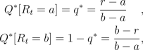
for
any time t.
Hint: Recall that the probability of an event
must
be a number between 0 and 1.
- What happens if p=0
or p=1?
- Verify the result given in d)
for the Examples given in the previous
lessons.
Important note: The justification of
each of the steps above does not have to be necessarily formal. A more
formal justification would require some background in mathematical
proofs and abstract concepts of probability which are out of the scope
of these lessons. However, the statement and consequences of the First
Fundamental Theorem of Asset Pricing should become clear after facing
these problems.